The Prehistory of Computing, Part I
What is a computer, really? Where did it come from? When did we realize we could trick rocks into doing our math homework for us?
In this two-part series, I’ll cover the origin and early history of computing and computer science, starting in prehistoric Africa and ending in Victorian-era England. Not exhaustively (because that would require an entire book) but selectively, highlighting the most interesting innovations and focusing on the untold (or at least less well known) stories. If I do my job right, you’ll practically hear a little “Level Up!” chime as the human race unlocks a new ability with each discovery.
Let’s start with the oldest evidence of computation I’m aware of.
The Ishango Bone
The Ishango Bone is a scraped and polished mammal bone, four inches (10 cm) long and probably around 20,000 years old. Divided into three separate columns are sixteen groups of short, parallel, evenly spaced notches which could only have been made with a sharp stone knife:
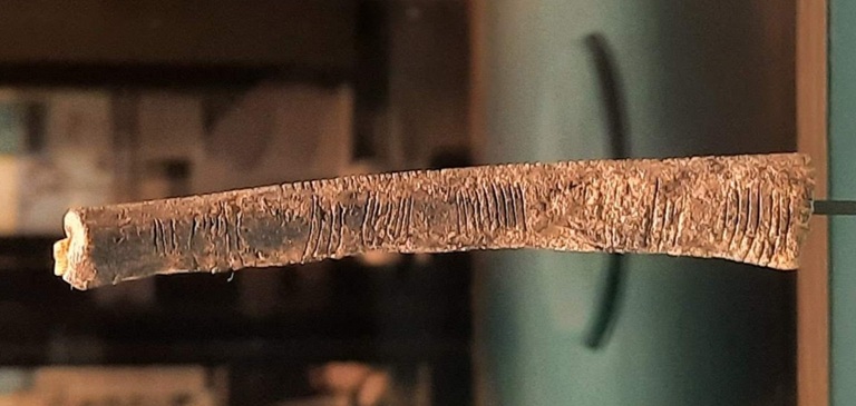
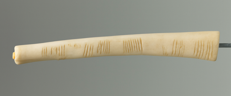
It’s quite hard to see the notches in the above picture, so here’s an AI recreation of what it would have looked like when new:
Archaeologists have found plenty of tally sticks at dig sites around the world, but what makes this one special are the numbers encoded in the grouped tally marks. There are three series of numbers, carved into three separate sides:
- 3, 6, 4, 8, 10, 5, 5, 7
- 11, 13, 17, 19
- 11, 21, 19, 9
It’s not hard to spot the patterns:
- In the first series, we see many examples of doubling and halving.
- In the second, we see every prime number between 10 and 20.
- In the third, two pairs of numbers each differing by 10.
Is this just pareidolia? I don’t think so. If we apply Tenenbaum’s “number game” approach, it becomes clear that it would be extraordinarily unlikely for so many meaningful patterns to appear, even when we consider the larger hypothesis space of other patterns we also would have found “meaningful” (tripling, powers of two, Fibonacci sequences, etc.) In particular, the doubling and halving of the first series suggests that some kind of mathematical calculation is taking place, making the Ishango bone the oldest piece of evidence we have of humans using an external object for computation.
Cuneiform Tablets
Which brings us to the first computer: the clay tablet.
Operation is simple: you press into the soft, wet clay with a stylus to make cuneiform symbols. You can smooth it over and re-use it for scratch calculations, or bake it for permanent storage.
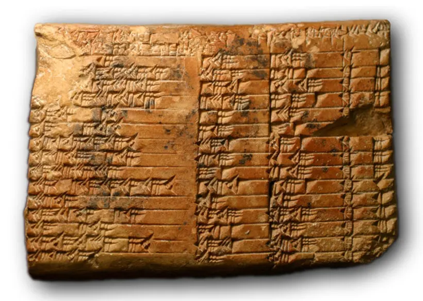
The above image is of Plimpton 322, a Mesopotamian clay tablet about four thousand years old, showing a table of known Pythagorean triples. This suggests that even at that early date, mathematics had progressed beyond counting and arithmetic and was already being studied for its abstract beauty.
“Wait,” I hear you ask, “how is poking mud with a stick a computer?” To see why, try the following 10-digit multiplication problem:
\[ \begin{array}{r} \hspace{8mm} 6847027875 \\ \times \hspace{3mm} 2463797377 \\ \hline \end{array} \]
All done? Were you able to do it in your head? Or did you resort to pen and paper?
Look, here’s the calculation shown in gory detail using the grade-school multiplication algorithm:
\[ \begin{array}{r} \hspace{8mm} 6847027875 \\ \times \hspace{3mm} 2463797377 \\ \hline 47929195125 \\ 479291951250 \\ 2054108362500 \\ 47929195125000 \\ 616232508750000 \\ 4792919512500000 \\ 20541083625000000 \\ 410821672500000000 \\ 2738811150000000000 \\ 13694055750000000000 \\ \hline 16869689318670883875 \\ \end{array} \]
To do it without recourse to external storage, you’d have to be able to store a minimum of 51 digits in working memory: ten each for the original factors, eleven more for the row you’re currently working on, and up to twenty for the running sum of rows. And that’s assuming that you compute the running total after each row! A running total saves space but wastes time; it’s much easier to write out all the rows first and then sum up the rows with carry. However, that approach requires at least 150 digits of working memory. Maybe some trained mnemonist could do that, but I sure couldn’t.
The human brain has about 7±2 digits of working memory, while a single tablet can easily hold hundreds. Thus, while the tablet can’t add even two digits together, and a human can’t store hundreds of digits in their head, the system composed of the human and the tablet together can. So while it may not seem like very advanced technology at first glance, by increasing the scribe’s effective working memory it trivializes calculations that would otherwise be impossible.
Papyrus
Before we move on, a brief word about papyrus. Why did I choose to talk about clay tablets instead of papyrus? After all, the Rhind and Moscow papyri are from roughly the same time period and also exhibit early abstract mathematics:
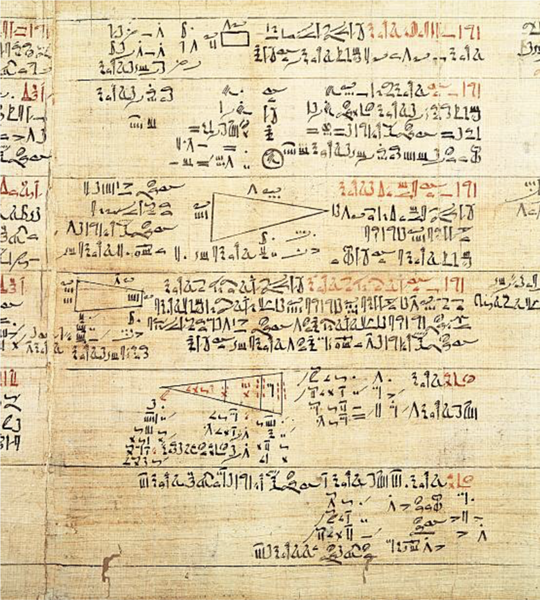
The reason is simple: papyrus was expensive and could not easily be reused. It would have been used for important records, but was far too valuable to use as scratch paper. Thus it would have been easily erasable clay tablets or ostraka that were actually used to carry out such calculations.
The Abacus
You’ve certainly seen an abacus before:
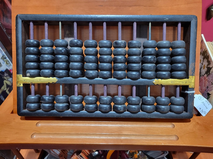
And you probably know that each column of beads encodes a single digit. But if you haven’t practiced using one, you probably don’t have any idea how fluent they can be.
Want to add two numbers? Your fingers already know the procedure: push these beads up, carry one over there, slide a few back down. Multiplication and division? Same story: the algorithms are encoded in muscle memory and can be executed very quickly, almost without conscious thought.
In other words, the abacus isn’t just a calculator; it’s a prototypical register machine.
Feynman tells this story about winning against an abacus in a cube root competition through a combination of pure luck and mathematical intuition. Afterwards, he concludes:
With the abacus, you don’t have to memorize a lot of arithmetic combinations; all you have to do is to learn to push the little beads up and down. You don’t have to memorize 9+7=16; you just know that when you add 9, you push a ten’s bead up and pull a one’s bead down. So we’re slower at basic arithmetic, but we know numbers.
It’s a funny anecdote, but I think his conclusion is backwards. Physicists often start with simple models that can be understood intuitively and solved exactly, and then add real-world complexity back in as a series of approximations to obtain numerically precise predictions. Naturally, Feynman views his approach (a moment of intuitive insight refined by later calculation) as superior. But had he been a computer scientist he would have realized that the very fact that the abacus operator was carrying out the calculation without thinking about the specific numbers involved shows that his approach is entirely algorithmic. If there’s one thing that Turing, Church, and Gödel can all agree on, it’s that rote, unthinking procedures are the essence of computation.
Ptolemy’s Almagest
Claudius Ptolemy was an astronomer active in 2nd-century CE Alexandria. His Almagest is the second most successful textbook of all time, surpassed only by Euclid’s Elements. It includes everything that was known at the time about the theory and practice of astronomy and continued to be widely used until the Copernican revolution in the 16th century.
There’s a tremendous amount that could be said about this influential book but we’ll focus on only a section that has direct relevance to our topic: the table of chords. If you want a more in-depth analysis of Almagest as a whole, the blog Following Kepler has done a multi-year deep dive into it.
A “chord” is a line segment which connects two points on a circle. The table of chords relates the opposite angle (in degrees) to the length of chord; essentially the same relationship as $\sin(\theta)$ in modern trigonometry with some scaling factors:
\[ \operatorname{chord}(\theta) = 2 R \sin\left(\frac{\theta}{2}\right) \]
Ptolemy precalculated this chord length for a large number of angles and published them as a table in his book. It wasn’t quite the first such table—Hipparchus had earlier developed a similar table of chords—but that table is now lost and is thought to have been less extensive than Ptolemy’s.
Here is a small sample of Ptolemy’s table, from a later Latin edition:
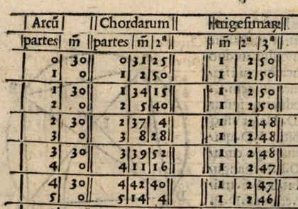
The column labeled “Arcu” is the angle; the “partes” is the angle in degrees and the “m” (for minuta) is one-sixtieth of a degree, so we can see each row represents a half-degree increment.
The column labelled “Chordarum” is the chord length given to a precision of about 1⁄3600, or about four decimal places. The table runs from $0^{\circ}$ to $180^{\circ}$ in half-degree increments so has about 360 rows. It would have been an impressive accomplishment in the 12th century, let alone the 2nd.
How did Ptolemy create this table? He used the theorem that bears his name to this day. Ptolemy’s theorem gives a relationship between the edges and diagonals of a cyclic quadrilateral:
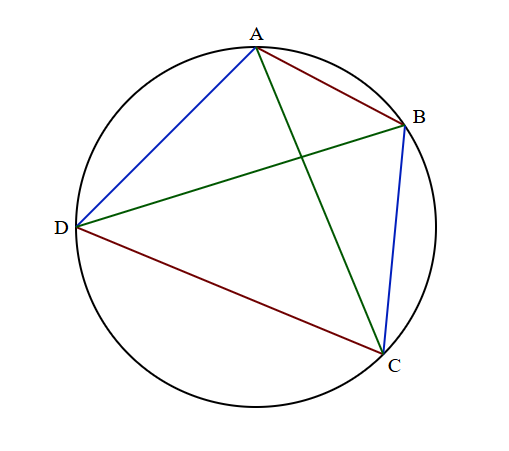
\[ \overline{AD} \times \overline{BC} + \overline{AB} \times \overline{CD} = \overline{AC} \times \overline{BD} \]
While seemingly elegant, it’s probably not at all obvious at first glance how this could have any practical use. It turns out, though, that it’s a powerful Swiss army knife for working with angles and chord lengths. To see how, let’s translate it into trigonometry so that it’s more recognizable to modern readers.
We do this by setting up the quadrilateral in a special way. We’ll choose $B$ and $D$ to be exactly opposite on the circle, and the diameter $\overline{BD}$ to be exactly one. Then we consider two angles, $\alpha$ and $\beta$, on opposite sides of this line:
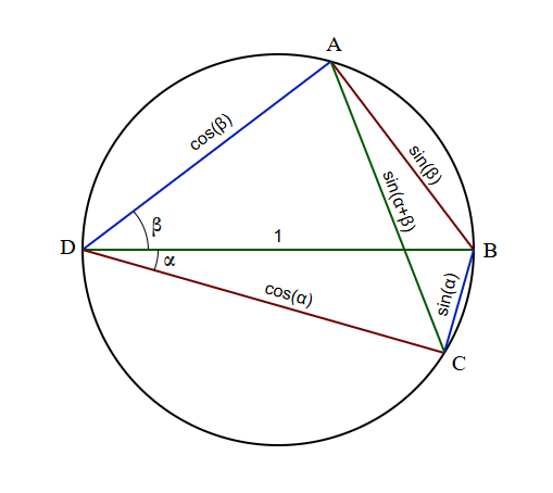
By the inscribed angle theorem, $\angle DAB$ and $\angle DCB$ are both right angles. That gives us two right triangles with hypotenuse $1$, so we can easily label the edge lengths as $\overline{BC} = \sin(\alpha)$, $\overline{AD} = \cos(\beta)$ and so on.
Now we can apply Ptolemy’s theorem. Since we chose $\overline{DB} = 1$, the right-hand side is just $\overline{AC}$. By the law of sines, $\overline{AC} = \sin(\alpha+\beta)$. Thus Ptolemy’s theorem gives us the angle addition formula:
\[ \sin(\alpha{+}\beta) = \sin(\alpha) \cos(\beta) + \cos(\alpha) \sin(\beta) \]
It’s this theorem that allowed Ptolemy to build out his table. He first calculated $\sin(1^{\circ})$ and $\sin(½^{\circ})$ and repeatedly added them together starting from the nearest known value (such as $\sin(30^{\circ}) = ½$) until the entire table was filled in.
Perhaps this is the point where you leap up from your chair and loudly complain, “how is this a computer? It’s not even a machine! It’s just a book!”
But a table is a computing device, just as much as a TI-85. It’s an external object that greatly reduces the time it takes to perform a calculation. Even modern computers routinely trade space for time with lookup tables and caches.
How did Ptolemy decide on four decimal places? Why not three or five? He must have known, probably through long experience, that after the handful of calculations involved in finding the position of a planet you’d still be left with three sig figs—enough to actually find the object in the sky. Such considerations anticipate modern numerical analysis.
The Sector
This device is called a sector:
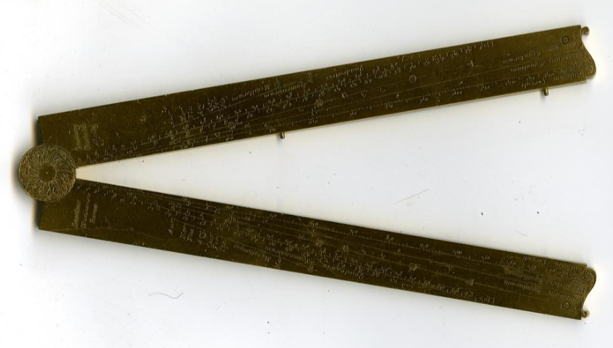
It seems kind of silly—it’s just a hinge—but it’s much more useful than it first appears. The sector translates angles, for which there are few useful tools, into distances, which can easily be manipulated with a compass.
The Smithsonian has an extensive collection of historical sectors, from which the above image is borrowed.
Galileo produced and sold a sector described in his 1606 book The Operations of the Geometric and Military Compass. His version included multiple scales in an attempt to squeeze as many useful functions into a single device as possible. It was, in a word, the scientific calculator of his day.
Chris Staecker has a good video demonstrating in detail the use of this specific sector for those who want to go into the details:
I want to draw attention to one scale in particular on Galileo’s sector, the C scale. The C scale is just a physical representation of Ptolemy’s table of chords. Open the sector to any angle and measure the distance across the sector with a compass; that’s the chord length. Pick up the compass and move it to the C scale on the sector; the value you read off is the angle in degrees. This process can be reversed as well, allowing you to open the sector to a particular angle that you only know as a number of degrees.
The disadvantage of using a sector for this purpose when compared to Ptolemy’s table is that you only get two or three sig figs, which is often sufficient for practical navigation work but not necessarily for precise astronomy. The advantage, of course, is that the operation is far more convenient than consulting a table.
We’ll see this tension between precision and computation time again when we discuss the logarithm, but first I want to spend a little time on one of the underappreciated giants of early computation.
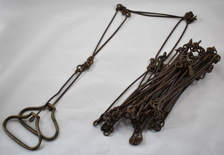
Edmund Gunter
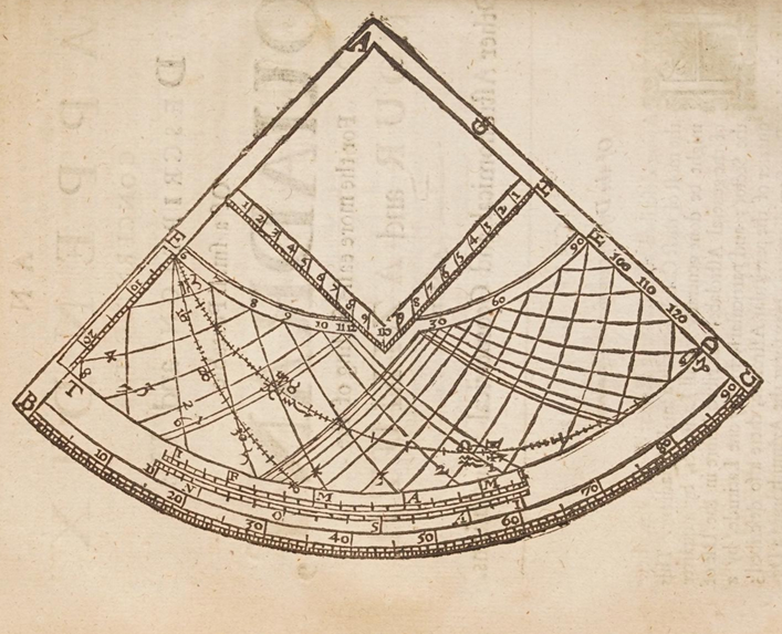
Edmund Gunter was a prolific inventor and proponent of practical computing devices, tables, and techniques. Many of his inventions and incremental improvements can be found in the posthumously published Works of Edmund Gunter. A few of the more famous are Gunter’s quadrant, a kind of astrolabe:
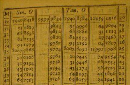
A table of trig functions given to an unprecedented seven decimal places of precision:
Gunter’s chain, used by surveyors to measure distances over rough terrain which continued in common use until surprisingly recently:
And numerous others. Really, just go flip through his book; it’s freely available in full on the Internet Archive.
But the main reason I bring him up is so I can relate this anecdote which I think tells us a lot about how computation was viewed until quite recently, before Turing et al. put it on a respectable academic footing:
[Gunter] brought with him his sector and quadrant, and fell to resolving triangles and doing a great many fine things. Said the grave knight [Savile], “Do you call this reading of geometry? This is showing of tricks, man!”, and so dismissed him with scorn, and sent for Henry Briggs.
This quote stood out for me because it highlights the extent to which his contemporaries fixated on theory and devalued computation, a theme we’ll return to later.
The Logarithm
The next leg of our journey is the logarithm, and in particular the two competing (or perhaps complementary) ways of materializing it: the log table and the slide rule.
The logarithm has its origin in an almost offhand comment by Michael Stifel on the connection between exponents and arithmetic/geometric series in his book Arithmetica Integra:
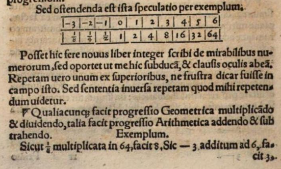
The second comment under the table translates to, “Just as geometric progression operates by multiplication and division, arithmetic progression follows addition and subtraction.” The table itself shows several examples of negative and positive exponents of 2, clearly illustrating the point.
In modern notation, we would write: \[ \log(xy) = \log(x) + \log(y) \]
The power of this statement—the magic really—is that addition and multiplication are far more closely related than anyone had guessed. The practical relevance to computation is that addition and subtraction are considerably faster and easier than multiplication or long division… so if they’re basically the same thing, why not do it the easy way?
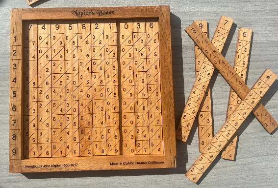
John Napier
Napier had already been searching for a way to make multiplication faster, and had had some success with a device called Napier’s bones:
We don’t know if Napier took inspiration from Stifel or not; Arithmetica Integra was a very famous book (it introduced exponents and negative numbers) so perhaps Napier had read it, or perhaps he developed the idea completely independently. But at some point he grasped the importance of the logarithm and how it could be used to efficiently perform multiplication.
He then spent an unknown number of hours in painstaking calculation over the next twenty years working out his tables to seven decimal places in a book he called the Mirifici Logarithmorum Canonis Descriptio, or the Description of the Wonderful Canon of Logarithms, published in 1614.
After a brief description of how to use the table, the remaining 90 pages of the book all look like this:
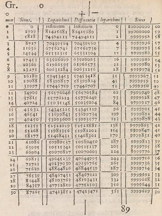
They give the logarithms (and closely related sines) to seven decimal places.
Napier’s book was a success and was immediately put to good use by scientists such as Johannes Kepler, who referred to it as a “happy calamity” because its timely publication saved him an enormous amount of effort in the construction of his own planetary tables.
Napier’s table of logarithms was a monumental breakthrough. It was a personal triumph: the glorious marriage of genius and industry. It attracted immediate and widespread acclaim. And it was obsolete almost from the moment the ink was dry.
Henry Briggs
Napier had made one unfortunate decision in his table; he implicitly chose a base of $\frac{1}{e}$ and a scale factor of $10^7$:
\[ n(x) = -10^7 \ln\left(\frac{x}{10^7}\right) \]
I say “unfortunate” because this convention adds an ugly magic number to every multiplication operation:
\[ n(xy) = n(x) + n(y) - 161180956 \]
This constant arises because $10^7 \ln\left(10^{7}\right) \;\approx\; 161180956.509\ldots$ Not a huge deal, but it does add an extra step to every single calculation.
It was Henry Briggs (the same one mentioned in the Edmund Gunter anecdote above) who realized that this constant could be eliminated entirely. He proposed what we would today call the base 10 logarithm:
\[ \log_{10}(xy) = \log_{10}(x) + \log_{10}(y) \]
Briggs discussed his idea with Napier, and then spent several years working out the new and improved table by hand, ultimately publishing it as the Arithmetica Logarithmica in 1624. It included 30,000 rows and gave its results to fourteen decimal places.
The logarithm revolutionized computation. Anyone who needed to multiply, divide, or find roots of numbers to a high degree of precision could now do so quickly and reliably. There was only one problem with the method: very often, one needed only a handful of significant figures, for which purposes flipping through the lengthy tables was overkill. What was needed was some convenient way to do quick-and-dirty calculations.
The Slide Rule
I can’t really do justice to the full history of the slide rule, which saw many improvements and incremental innovations during the three centuries in which it was in widespread use, but will at least sketch its origin story.
Edmund Gunter was the first to print Napier’s log scale on a ruler:
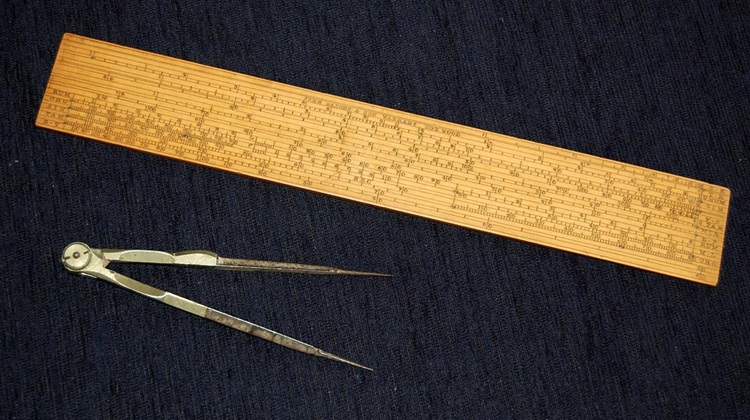
In conjunction with a compass, it could be used in a conceptually similar way to a log table. To multiply two numbers $x$ and $y$, first find where the number $x$ is printed on the log scale and use a compass to measure the distance to the origin. This distance is roughly $\log(x)$. Then find the point where $y$ is printed. Pick up the compass, pinching its pivot so that it retains its length, and add that distance to the point for $y$. Since these two lengths added together make $\log(x) + \log(y) = \log(xy)$, the number printed on the scale at this new point is $x \times y$.
This isn’t terribly precise; maybe two or three sig figs in practice. But it’s a lot faster than flipping through 90 pages of tables.
It was William Oughtred who took the next step and gave us the first recognizable slide rule by simply placing two Gunter rules next to each other. This eliminated the need for a compass and made the whole operation quicker and more precise. Oughtred’s original slide rule does not survive, so here is a much later version:
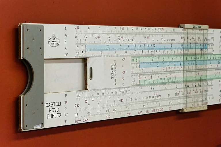
This later version features many innovations and ergonomic conveniences, such as the cursor (a simple addition which greatly improves precision) and the addition of other scales (for trigonometric functions, etc.) reminiscent of the multiple scales engraved onto Galileo’s sector.
Perhaps Oughtred would not have appreciated being remembered as “the inventor of the slide rule” as he believed that mathematical proof was far more important than mere calculation, which he likened to a juggler’s tricks:
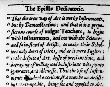
An attitude which echoes Savile’s dismissal of Gunter. It’s easy with the benefit of hindsight to view this as naïve; after all, we know how important the slide rule turned out to be, an importance that is only magnified when we view it as a stepping stone to the modern computer. But none of this would have been obvious even to the best minds of the time. Living in an essentially agrarian society, writing with quill pens on parchment by candlelight, caught between the church and feudal lords in a world of handcrafted objects, they could not have conceived the value that a pocket slide rule would have to a 20th century engineer.
“Some of the greatest discoveries consist mainly in the clearing away of psychological roadblocks which obstruct the approach to reality; which is why, post factum, they appear so obvious.”
—Arthur Koestler
Conclusion
In part II of this series, we’ll cover the first mechanical calculators, as well as some of the theory that laid the foundation for modern computer science.