Complex Numbers in R, Part I

Pythagorean Triples

Let’s start with a problem which could be solved in other ways, but is greatly simplified by the introduction of complex numbers that it almost seems magical.

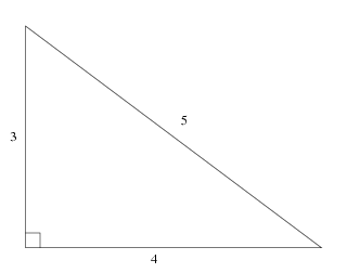
A Pythagorean triple is an integer solution to the Pythagorean equation:

\[ a^2 + b^2 = c^2 \quad\quad a,b,c \in \mathbb{N}^+ \tag{1} \]

You probably learned at least one of these in school – the famous 3, 4, 5 triangle:

In general Diophantine equations – which require integer solutions – can be quite hard to solve, so it might surprise you to hear that it’s almost trivially easy to write down an infinite of Pythagorean triples. Well, it’s easy if we use complex numbers, anyway.

A Gaussian integer is a complex number where both the real and imaginary parts are integers. The set of Gaussian integers is denoted by \(\mathbb{Z}[i]\) and is defined as:

\[ \mathbb{Z}[i] = \{ x + iy \mid x,y \in \mathbb{Z} \} \tag{2} \]

So one way of stating the problem of finding all Pythagorean triples is to find all Gaussian integers which are an integer distance away from the origin. The distance of a complex number from the origin is called its “norm” and denoted \(\lVert z \rVert\). We will call the set of Pythagorean triples \(T\) and define it as:

\[ T = \{ z \in \mathbb{Z}[i] \mid \lVert z \rVert \in \mathbb{Z} \} \tag{3} \]

Now, in general the norm of Gaussian integer will be the square root of an integer (the integer \(x^2 + y^2\) to be precise.) Therefore if we square a Gaussian integer, it will have an integer norm and therefore represent a Pythagorean triple!

\[ \forall z \in \mathbb{C}, z \in \mathbb{Z}[i] \implies z^2 \in T \tag{4} \]

So that’s a pretty good start: just a few minutes work, and we’ve already found an infinite number of Pythagorean triples, and we have a computationally trivial way of constructing new triples: we simply pick any two positive integers \(x\) and \(y\) and then square the complex number \(x + iy\).

Before address the more difficult question of whether or not we’ve found all possible Pythagorean triples using this construction, let’s switch over to R and write some code to capture our solution so far.

Gaussian Integers in R

Our algorithm first requires us to pick pairs of positive integers. Just to be thorough, we’ll take all such pairs up to an arbitrary threshold.

Now, if we wanted just one or two complex numbers, we could use the literal syntax:

triples <- c( 3+4i, 5+12i, 9+12i )

But since want to construct them in bulk, we’ll use the complex() constructor. This constructor is vectorized: by passing in two vectors of equal length we can construct a one-dimensional vector of complex numbers.

n = 400
grid <- expand.grid(u=1:(2*n), v=1:(2*n))
grid <- grid[ grid$u > grid$v, ]
gaussian_integers <- complex(real=grid$u, imaginary=grid$v)

Per the theoretical discussion above, we can generate Pythagorean triples by simply squaring these. All primitive math functions in R work just as well on complex numbers: exp, log, sin, cosand of course the power operator ^:

triples <- gaussian_integers^2

# display the 10 with the smallest norm
cat( triples[order(Mod(triples))][1:10], sep="\n")

# 3+4i
# 8+6i
# 5+12i
# 15+8i
# 12+16i
# 7+24i
# 24+10i
# 21+20i
# 16+30i
# 35+12i

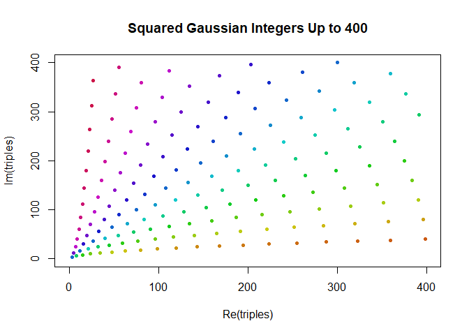
Did it work? We’re certainly seeing some familiar pairings there, like \(5+12i\) which maps to well-known triple \((5,12,13)\). To visualize them, we can simply pass our complex vector to R’s plot() function – it will conveniently plot them in the complex plane for us!

triples <- triples[ Re(triples) <= n & Im(triples) <= n ]

# helper function to colorize complex points by their angle.
argcolor <- function(z) hsv(Arg(z)*2/pi, s=0.9, v=0.8)

plot(
  triples, 
  col=argcolor(triples),
  pch=20,
  xlim=c(0,n),
  ylim=c(0,n),
  main=paste("Squared Gaussian Integers Up to", n)
)

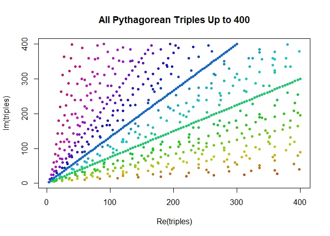
Now it turns out that our algorithm does not, in fact, generate all possible triples. For example, multiples are missing: if \((3,4,5)\) is a triple, then \((6,8,10)\) should be a triple, and \((9,12,15)\) should be a triple, and so on. So we have to expand our set to have all multiples.

multiples <- lapply(1:(floor(n/3)), function(m) triples*m)
triples <- unique(do.call(c, multiples))

It also turns out that in the special case where both integers are even we can divide by two and get a new triple that was missed by the initial net we cast. But that’s the end of the special cases – with this final rule in place, we’re now guaranteed to hit every Pythagorean triple.

halves <- triples[ Re(triples) %% 2 == 0 & Im(triples) %% 2 == 0 ] / 2
triples <- unique(c(triples, halves))

Now all we need to is clean up duplicates and duplicate along the mirror line of symmetry…

triples <- triples[ Re(triples) <= n & Im(triples) <= n]
triples <- c(triples, complex(real=Im(triples), imaginary=Re(triples)))

..and we’re finally ready to visualize the real solution.

plot(triples, col=argcolor(triples), pch=20)
title(paste("All Pythagorean Triples Up to", n))

A Closer Look

That’s too many to really understand, although there are definitely patterns emerging. Let’s zoom in and just plot a small region,but with more detail.

small_n = 25
small_triples <- triples[ Re(triples) < small_n & Im(triples) < small_n ]
small_triples <- small_triples[ order(Mod(small_triples), decreasing=TRUE) ]

# plot points
plot(
  small_triples, 
  pch=20,
  ylim=c(0,small_n), 
  xlim=c(0,small_n),
  ylab="b", xlab="a")

# add triangles. Can't rely on automatic complex plane plotting here.
segments(
  Re(small_triples), Im(small_triples), 
  0, 0, 
  col=argcolor(small_triples))
segments(
  Re(small_triples), Im(small_triples), 
  Re(small_triples), 0, 
  col=argcolor(small_triples))
segments(
  Re(small_triples), 0, 
  0, 0, 
  col=argcolor(small_triples))

# points again, so that they're in the foreground.
points(small_triples, pch=20, col=argcolor(triples), cex=1)

# text label for the points
text(
  x=small_triples + 1i, 
  cex=0.8,
  labels=paste0(
    "(", 
    Re(small_triples), 
    ",",
    Im(small_triples),
    ",",
    Mod(small_triples),
    ")"
  )
)
title(paste("Pythagorean Triples Up to", small_n))

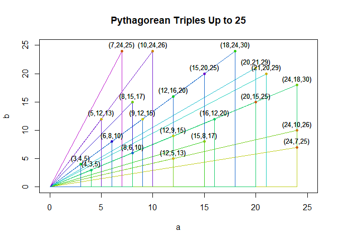
On the zoomed in view we can see each Pythagorean triple represented as a right triangle; that the integer multiples of solutions form a series of similar triangles; and that there’s a strong symmetry with every triple \((a,b,c)\) having a partner \((b,a,c)\) which is its mirror reflection about the like \(y=x\).

From the zoomed out view we can see that the region close to either the x-axis or the y-axis is essentially devoid of solutions and that it looks as if triples actually get less dense as we move away from the origin.

By the way, this last observation about triples thinning out as we move away from the origin can be understood and quantified by once again using the complex plane. Triples are more or less the squares of Gaussian integers; we can say the number of triples with norm less than \(r\) is roughly proportional to the number of Gaussian integers in the first quadrant and inside a circle with radius \(\sqrt{r}\), which is roughly proportional to the area of the quarter-circle of radius \(\sqrt{r}\), which is \(\frac{\pi r}{4}\) or very roughly just \(r\).

Next Time

In this first part of a planned series on complex numbers in R, we dipped our toes in the water by explicitly creating some complex numbers and manipulating them. We demonstrated the most important functions for working specificly with complex numbers such as Re(), Im(), Mod(), Arg(), and complex() but we emphasized that most built-in functions such as exp() and operators such as * and ^ work correctly with complex numbers and implement the natural analytic continuation of their equivalents on the real numbers. Finally, we showcased R’s ability to plot on the complex plane.

Next time in Part II, we will discuss in more depth some scenarios where complex numbers arise naturally from the problem itself and cannot be reasonably avoided, while continuing to demostrate more advanced aspects of R’s complex number functionalty.