A Fairly Fast Fibonacci Function

def naive_fib(n):
    if n < 2:
        return n
    else:
        return naive_fib(n-1) + naive_fib(n-2)

from functools import lru_cache

@lru_cache(100)
def memoized_fib(n):
    if n < 2:
        return n
    else:
        return memoized_fib(n-1) + memoized_fib(n-2)

def table_fib(n):
    if n < 2:
        return n
    table = [-1] * (n+1)
    table[0] = 0
    table[1] = 1
    for i in range(_2, n+1):
        table[i] = table[i-1] + table[i-2]
    return table[n]

def iterative_fib(n):
    previous, current = (0, 1)
    for i in range(2, n+1):
        previous, current = (current, previous + current)
    return current

Matrix Form

There exist several closed-form solutions to Fibonacci sequence which gives us the false hope that there might be an \(\mathcal{O}(1)\) solution. Unfortunately they all turn out to be non-optimal if you want an exact solution for a large \(n\). We will use to so-called “matrix form” instead, which we will now describe in some detail.

Recall that the \(n\)-th Fibonacci number is given by the recurrence relation:

\[ \begin{align} F_0 &= 0 \\ F_1 &= 1 \\ F_n &= F_{n-1} + F_{n-2} \end{align} \]

Define the first Fibonacci matrix to be:

\[ \mathbf{F}_1 = \begin{bmatrix} 1 & 1 \\ 1 & 0 \end{bmatrix} \]

And define the \(n\)-th Fibonacci matrix to be the \(n\)-th power:

\[ \mathbf{F}_n = \mathbf{F}_1^n \]

I didn’t just pluck this out of thin air - there’s a general way to turn any linear recurrence relation into a matrix which I’ll describe in a moment. But first let’s prove the following theorem, which justifies our definition:

\[ \forall n \in \mathbb{N}, \mathbf{F}_n = \begin{bmatrix} F_{n+1} & F_n \\ F_n & F_{n-1} \end{bmatrix} \]

We proceed by induction. For the case of \(n = 1\), the theorem is true by inspection because we know \(F_0 = 0\) and \(F_1 = F_2 = 1\).

Suppose it is true for \(n-1\). Then we have:

\[ \mathbf{F}_n = \mathbf{F}_1^{n} = \mathbf{F}_1^{n-1} \mathbf{F}_1 = \begin{bmatrix} F_n & F_{n-1} \\ F_{n-1} & F_{n-2} \end{bmatrix} \begin{bmatrix} 1 & 1 \\ 1 & 0 \end{bmatrix} \]

Multiplying these two matrices, we have:

\[ \mathbf{F}_n = \begin{bmatrix} F_n + F_{n-1} & F_{n} \\ F_{n-1} + F_{n-2} & F_{n-1} \end{bmatrix} \]

We can use the Fibonacci definition twice (once for each element of the first column) to get:

\[ \mathbf{F}_n = \begin{bmatrix} F_{n+1} & F_{n} \\ F_{n} & F_{n-1} \end{bmatrix} \]

Therefore if the theorem is true for \(n-1\), it is also true for \(n\). We have already shown it is true for \(n = 1\), so by mathematical induction it is true for all \(n \geq 1\). Q.E.D.

A brief word about where this matrix representation came from. Wikipedia has a good explanation for how any linear recurrence relation can be expressed in matrix form and I’ve described it myself in a prior article. Essentially, we use the first dimension to store the current value, and the rest of the vector as shift registers to “remember” previous states. The recurrence relation is encoded along the first row and the ones along the subdiagonal roll the history forward. It’s actually easier to see in higher dimensions, so here’s an example of encoding a linear recurrence relationship which uses the four most recent numbers instead of just two:

\[ y_{n+1} = c_0 y_n + c_1 y_{n-1} + c_2 y_{n-2} + c_3 y_{n-3} \\ \iff \\ \begin{bmatrix} y_{n+1} \\ y_{n} \\ y_{n-1} \\ y_{n-2} \\ y_{n-3} \\ \end{bmatrix} = \begin{bmatrix} c_0 & c_0 & c_1 & c_2 & c_3 \\ 1 & 0 & 0 & 0 & 0 \\ 0 & 1 & 0 & 0 & 0 \\ 0 & 0 & 1 & 0 & 0 \\ 0 & 0 & 0 & 1 & 0 \\ \end{bmatrix} \begin{bmatrix} y_n \\ y_{n-1} \\ y_{n-2} \\ y_{n-3} \\ y_{n-4} \\ \end{bmatrix} \]

If we squint at \(\mathbf{F}_1\), we can see it has this form too: the first row is \([ 1 \,\, 1 ]\) because recurrence relation is simply the sum of the previous two, while the second row \([ 1 \,\, 0 ]\) contains the \(1\) on the subdiagonal which “remembers” the previous value. The effect is to advance the state of the algorithm in almost the exact same way as the interative_fib() above:

\[ \begin{bmatrix} 1 & 1 \\ 1 & 0 \end{bmatrix} \begin{bmatrix} F_n \\ F_{n-1} \end{bmatrix} = \begin{bmatrix} F_n + F_{n-1} \\ F_{n} \end{bmatrix} = \begin{bmatrix} F_{n+1} \\ F_{n} \end{bmatrix} \]

At first this may not seem at all helpful. But by framing the problem as taking the exponent of a matrix instead of repeated addition, we can derive two much faster algorithms: a constant time \(\mathcal{O}(n)\) approximate solution using eigenvalues, and a fast \(\mathcal{O}(n \log n)\) exact solution.

Eigenvalue Solution

Note that the matrix \(\mathbf{F}_1\) is symmetric and real-valued. Therefore it has real eigenvalues which we’ll call \(\lambda_1\) and \(\lambda_2\). The eigenvalue decomposition allows us to diagonalize \(\mathbf{F}_1\) like so:

\[ \mathbf{F}_1 = \mathbf{Q} \mathbf{\Lambda} \mathbf{Q}^T = \mathbf{Q} \begin{bmatrix} \lambda_1 & 0 \\ 0 & \lambda_2 \end{bmatrix} \mathbf{Q}^T \]

Writing \(\mathbf{F}_1\) in this form makes it easy to square it:

\[ \begin{align} \mathbf{F}_1^2 & = \mathbf{Q} \mathbf{\Lambda} \mathbf{Q}^T \mathbf{Q} \mathbf{\Lambda} \mathbf{Q}^T \\ & = \mathbf{Q} \mathbf{\Lambda}^2 \mathbf{Q}^T \\ & = \mathbf{Q} \begin{bmatrix} \lambda_1^2 & 0 \\ 0 & \lambda_2^2 \end{bmatrix} \mathbf{Q}^T \end{align} \]

or to raise it to an arbitrary power:

\[ \mathbf{F_n} = \mathbf{F}_1^n = \mathbf{Q} \mathbf{\Lambda}^n \mathbf{Q}^T = \mathbf{Q} \begin{bmatrix} \lambda_1^n & 0 \\ 0 & \lambda_2^n \end{bmatrix} \mathbf{Q}^T \]

We can calculate the two eigenvalues analytically by solving the characteristic equation \((1-\lambda)\lambda - 1 = 0\). Since this is a quadratic polynomial, we can use the quadratic equation to obtain both solutions in closed form:

\[ \begin{align} \lambda_1 & = \frac{1 + \sqrt{5}}{2} \\ \lambda_2 & = \frac{1 - \sqrt{5}}{2} \end{align} \]

Where the largest eigenvalue is in fact \(\phi\), the golden ratio. The matrix formulation is an easy way to see famous connection between the Fibonacci numbers and \(\phi\). To calculate \(F_n\) for large values of \(n\), it suffices to calculate \(\phi^n\) and then do some constant time \(\mathcal{O}(1)\) bookkeeping, like so:

import numpy as np

def eigen_fib(n):
    F1 = np.array([[1, 1], [1, 0]])
    eigenvalues, eigenvectors = np.linalg.eig(F1)
    Fn = eigenvectors @ np.diag(eigenvalues ** n) @ eigenvectors.T
    return int(np.rint(Fn[0, 1]))

So there you have it – a \(\mathcal{O}(1)\) algorithm for any Fibonacci number. There’s just one tiny little problem with it: \(\phi\), being irrational, is not particularly convenient for numerical analysis. If we run the above Python program, it will use 64-bit floating point arithmetic and will never be able to precisely represent more than 15 decimal digits. That only lets us calculate up to \(F_{93}\) before we no longer have enough precision to exactly represent it. Past \(F_{93}\), our clever little “exact” eigenvalue algorithm is good for nothing but a rough approximation!

Now, we could use a high precision rational numbers, but that approach turns out to always require strictly more space and time that just sticking to integers. So, abandoning the eigenvalue approach on the garbage heap of ivory tower theory, let’s turn our attention to simply calculating the powers of an integer matrix.

Fast Exponentiation

So far, all we’ve done is reformulate our problem so that instead of calculating \(n\) terms in a sequence using simple addition, we now have to multiply \(n\) matrices together. We’ve made things worse! Multiplication is slower than addition, especially for large numbers, and computing the production of two \(2 \times 2\) matrices requires eight multiplications!

Remain calm. There’s a trick to calculating large powers quickly. Imagine we want to calculate \(x^n\) where \(n\) is a power of two: \(n = 2^m\). If we square \(x\), then square it again, and keep doing that \(m\) times, we get

\[ ((x^2)^2...)^2 = x^{2^m} = x^n \]

In other words, we only need to perform \(m = \log_2 n\) matrix multiplications to calculate \(x^n\).

We can generalize this to calculate any large power \(n\) (not necessary a power of two) by first finding the largest power of two less than \(n\) and factoring it out:

\[ x^n = x^{2^m} x^{n-2^m} \]

The left factor can be calculated by repeated squaring and the right factor by can calculated by recursively applying the same trick. However, we will never need to do that more than \(\log_2 n\) times and each time the power of two gets smaller.

The upshot is that we can calculate \(x^n\) in \(\mathcal{O}(\log n)\) multiplications. This is mostly commonly seen in cryptography such as the RSA algorithm and Diffie-Hellman key exchange where it is done modulo some large but fixed sized integer, making all the multiplications roughly equal cost. Here, we are using multiple precision integers which are doubling in size with each multiplication. That means abstract “multiplications” are the wrong thing to count. We won’t get \(\mathcal{O}(\log n)\) runtime performance because the top multiplications keep getting more expensive. Nevertheless, the squaring by exponentiation trick hugely reduces the amount of work we have to do relative to the naive iterative solution.

Matrix Implementation

Fun fact: Python has multiple precision baked in. If if an arithmetic operation on Python’s int() type exceed the normal limits of a 64-bit integer, Python will transparently substitute a high precision type. This makes Python a convenient language for working with very large numbers.

Now, we could just rely on NumPy’s matrix multiplication, like so:

F1 = numpy.array([[1,1],[1,]], dtype='object') 
numpy.linalg.matrix_power(F1, n)

This works. (Although strangely enough matrix multiplication with the @ operator doesn’t work when dtype='object'.) As much as love numpy though, I don’t think we need to drag it in as a dependency just to multiply \(2 \times 2\) matrices when we’re not even using native integer types.

Plus, we’ll see see in a second that there are some optimizations we can make that wouldn’t be possible if we let NumPy handle everything for us. So for now, let’s implement the naive matrix algorithm in native Python; we’ll come back and refactor in the next section.

First, for testing and benchmarking purposes, we’ll write a non-optimized version that just implements matrix powers in a straightforward way:

def matrix_multiply(A, B):
    a, b, c, d = A
    x, y, z, w = B
    
    return (
        a*x + b*z,
        a*y + b*w,
        c*x + d*z,
        c*y + d*w,
    )

def naive_matrix_power(A, m):
    if m == 0:
        return [1, 0, 0, 1]
    B = A
    for _ in range(m-1):
        B = matrix_multiply(B, A)
    return B

def naive_matrix_fib(n):
    return naive_matrix_power(F1, n)[1]

But we’ll immediately want to move on to a version which implements the fast exponentiation by repeated squares described above:

def matrix_power(A, m):
    if m == 0:
        return [1, 0, 0, 1]
    elif m == 1:
        return A
    else:
        B = A
        n = 2
        while n <= m:
            # repeated square B until n = 2^q > m
            B = matrix_multiply(B, B)
            n = n*2
        # add on the remainder
        R = matrix_power(A, m-n//2)
        return matrix_multiply(B, R)

F1 = [1, 1, 
      1, 0]

def matrix_fib(n):
    return matrix_power(F1, n)[1]

Implicit Matrix Form

The above has reasonably good asymptotic performance but it bothers me that it’s doing 8 multiplications each time. Luckily, because all Fibonacci matrices are of a special form, we really only need to keep track of two elements in the right-hand column of the matrix. I call this this the “implicit matrix form.” Here is a Fibonacci matrix described with just two numbers, \(a\) and \(b\):

\[ \mathbf{F}_n = \begin{bmatrix} \color{lightgrey} a + b & a \\ \color{lightgrey} a & b \end{bmatrix} \]

We can easily work out closed forms for multiplying and squaring matrices in this form. While the full expressions are a little complex - we never actually need to explicitly calculate the left-hand column, a fact I will indicate by graying those columns out:

\[ \begin{align} \begin{bmatrix} \color{lightgrey} a + b & a \\ \color{lightgrey} a & b \end{bmatrix} & \begin{bmatrix} \color{lightgrey} x + y & x \\ \color{lightgrey} x & y \end{bmatrix} & = \begin{bmatrix} \color{lightgrey} a(2x+y) + b(x+y) & a(x+y) + bx \\ \color{lightgrey} a(x+y) + bx & ax + by \end{bmatrix} \\ & \begin{bmatrix} \color{lightgrey} a + b & a \\ \color{lightgrey} a & b \end{bmatrix}^2 & = \begin{bmatrix} \color{lightgrey} 2a^2 + 2ab + b^2 & a^2 + 2ab \\ \color{lightgrey} a^2 + 2ab & a^2 + b^2 \end{bmatrix} \end{align} \]

Using the implicit matrix form, we can multiply two different Fibonacci matrices with just four multiplications, and we can squaring a matrix with only three! It’s only a constant time speed-up but every little bit helps.

def multiply(a, b, x, y):
    return x*(a+b) + a*y, a*x + b*y

def square(a, b):
    a2 = a * a
    b2 = b * b
    ab = a * b
    return a2 + (ab << 1), a2 + b2

def power(a, b, m):
    if m == 0:
        return (0, 1)
    elif m == 1:
        return (a, b)
    else:
        x, y = a, b
        n = 2
        while n <= m:
            # repeated square until n = 2^q > m
            x, y = square(x, y)
            n = n*2
        # add on the remainder
        a, b = power(a, b, m-n//2)
        return multiply(x, y, a, b)

def implicit_fib(n):
    a, b = power(1, 0, n)
    return a

It would of course be possible to derive these relationships without ever introducing the Fibonacci matrices, but I think they provides a valuable foundation for intuition. Without that foundation, the above program seems a little arbitrary.

You may be wondering why I square numbers as a*a instead of a**2 or pow(a, 2), and why I use ab<<1 instead of 2*ab or ab+ab to double them. The answer is simple - I benchmarked the various forms and found these expressions to be very slightly faster, at least when using large mpz() objects (which we’ll get to in a moment.)

Cython

Another thing to try – something which usually helps a lot – is to try converting our program to Cython.

Unfortunately, the one type that we want to use, Python’s native int() type, is represented by Cython as a C-style int - fixed precision signed integer. It doesn’t have Python’s ability to transparently handle large numbers. We can either use the native C long in which case we run into precision problems after \(F_{93}\), or we can continue to use the Python int() type in which case we gain only a modest speed up.

%%cython

cdef cython_multiply(a, b, x, y):
    return x*(a+b) + a*y, a*x + b*y

cdef cython_square(a, b):
    a2 = a * a
    b2 = b * b
    ab = a * b
    return a2 + (ab << 1), a2 + b2

cdef cython_power(a, b, int m):
    cdef int n = 2
    if m == 0:
        return (0, 1)
    elif m == 1:
        return (a, b)
    else:
        x, y = a, b
        while n <= m:
            # repeated square until n = 2^q > m
            x, y = cython_square(x, y)
            n = n*2
        # add on the remainder
        a, b = cython_power(a, b, m-n//2)
        return cython_multiply(x, y, a, b)
    
cpdef cython_fib(n):
    a, b = cython_power(1, 0, n)
    return a

print(cython_fib(103))

We still get a good boost for small numbers, but the benefit of this quickly becomes irrelevant for large numbers.

Never fret, though, because we can use something even better.

The GNU Multiple Precision Arithmetic Library

The GNU Multiple Precision Arithmetic Library, or GMP for short, is nothing short of a work of art. Often used for calculating \(\pi\) to a number of decimal places described as “silly” by their own documentation, GMP is able to add, multiply, divide and perform arithmetic on larger and larger numbers until your computer runs out of RAM. The multiplication algorithm used starts with Karatsuba - and then they get serious.

It’s almost embarrassingly easy to convert our algorithm to use GMP because the mpz() type is a drop-in replacement for int():

import gmpy2
from gmpy2 import mpz

def gmp_fib(n):
    a, b = power(mpz(1), mpz(0), mpz(n))
    return a

Note that we didn’t have to define the power() or multiply() functions again: this implementation re-uses the exact same functions we wrote for Python native types when implementing implicit_fib() above. Every Python function is a type-agnostic template function.

You may also wonder why the large integer type is called mpz: the “mp” is for “multiple precision”, just like the “MP” in “GMP,” while the “z” stands for \(\mathbb{Z}\), the conventional name for the set of integers. There is also mpq for the set of rationals \(\mathbb{Q}\) and so on.

Dynamic Programming Redux

The GMP version is really quite extraordinarily fast, but if we look at the call graph we can still see some redundant effort. It turns out that we are recalculating each power of two every time we need it, resulting in this ever widening tree-shaped DFG:

We can fix this with - you guessed it - dynamic programming! With dynamic programming, it’s a good idea to only cache the results of sub-problems which are likely to be re-used. Here, we can be reasonably certain that the only results worth caching are the powers of two, so we refactor that to its own function and apply memoization there.

# improve the algorithm slightly by caching
# and re-using powers of two. 
@lru_cache(100)
def dynamic_repeated_squares(a, b, n):
    # n must be a power of two. 
    if n == 0:
        return (0, 1)
    elif n == 1:
        return (a, b)
    return square(*dynamic_repeated_squares(a, b, n//2))
    
def dynamic_power(a, b, m):
    if m == 0:
        return (0, 1)
    elif m == 1:
        return (a, b)
    else:
        # hit the cache for powers of 2
        n = 2
        while n <= m:
            n = n*2
        n = n // 2
        x, y = dynamic_repeated_squares(a, b, n)

        # add on the remainder
        a, b = dynamic_power(a, b, m-n)
        return multiply(x, y, a, b)
    
def dynamic_fib(n):
    a, b = dynamic_power(mpz(1), mpz(0), mpz(n))
    return a

With the caching added for powers of two, we get a much smaller DFG, now an acyclic graph with no duplicate effort at all:

It should be clear from graph that in the worst case scenario, where \(n = 2^m -1\), the cached algorithm performs a maximum of \(2m\) multiplications, compared to the \(m(m-1)/2\) needed for the algorithm without caching. Despite this, the benefit of the cache is surprisingly minor: maybe 10% in practice. That’s because almost all the time is spent in a handful of very large multiplications – the smaller ones just don’t matter as much. “Logical multiplications” just isn’t the right operation to count. When dealing with multiple precision numbers we need to look at the number of bytes multiplied, and the number of bytes doubling with each multiplication. I’ve heard those two effects more or less cancel out and the final algorithm is \(\mathcal{O}(n \log n)\) but won’t venture to prove it myself. It seems to roughly hold empirically: every time \(n\) goes up by a factor of 10, time increases by about 20. (See the benchmarks below.)

C++ Fibonacci

Now that we’ve exhausted my ideas for algorithmic optimizations, there’s really only one thing approach left: micro-optimization. So far we’ve been working in Python, but Python has a reputation for being slow and we did see a small speed-up when we started using Cython. The GMP library is native to C; maybe a C or C++ program would eliminate all the Python overhead?

To find out, I ported the above logic pretty faithfully to C++, almost line-for-line:

// memoized version
ImplicitMatrix repeatedSquares(int n)
{
    // 0 squares means the original basis matrix f1
    static std::vector<ImplicitMatrix> cache = { {1, 0} };

    // repeatedly square as often as necessary.
    while (n >= cache.size() ) {
        cache.push_back( square(cache.back()) );
    }

    // the n-th element is always f1^n.
    return cache[n];
}

ImplicitMatrix power(
    const ImplicitMatrix& x,
    const bigint& m)
{
    if ( m == 0 ) {
        return {0, 1};
    } else if ( m == 1 ) {
        return x;
    }

    // powers of two by iterated squaring
    // ImplicitMatrix powerOfTwo = x;
    bigint n = 2;
    int n_squares_needed = 0;
    while ( n <= m ) {
        n = n*2;
        n_squares_needed++;
    //powerOfTwo = square(powerOfTwo);
    }
    ImplicitMatrix powerOfTwo = repeatedSquares(n_squares_needed);

    // recurse for remainder
    ImplicitMatrix remainder = power(x, m-n/2);

    return multiply(powerOfTwo, remainder);
}

I installed these libraries on Debian/Ubuntu like so:

sudo apt install libboost-all-dev libgmp-dev

The above program was built like so:

g++ -std=c++17 -O3 -o fib main.cpp -lgmp

Note that -O3 tells the compiler to apply maximum optimization to the program. That’s also why we need the volatile keyword - the optimizer notices my program doesn’t actually do anything and optimizes the whole thing away!

The results we mildly disappointing:

~/fib$ time ./fib 10000003

real    0m0.427s
user    0m0.360s
sys     0m0.060s

~/fib$ time ./fib 1000000003

real    1m24.088s
user    1m22.550s
sys     0m1.430s

If this is any faster than the Python version, it can’t be be measured. This result isn’t actually too surprising - at this point, 99.9% of computation time is spent in the GMP multiplication routines, and only a few microseconds are spent in Python. So we’re not going to squeeze any more performance out that way.

Final Python Fibonacci

Our performance testing has revealed something interesting - there is no one implementation which strictly dominates all the others over all possible inputs. The simple algorithms tend to win when \(n\) is small, while more complex algorithms are able to pull ahead when \(n\) is large.

A common way to squeeze as much performance as possible across all possible inputs is to use a hybrid algorithm which selects an algorithm from a family based on heuristics that estimate which should perform best in which regions. A hybrid solution is the Annie Oakley solution: “Anything you can do I can do better; I can do anything better than you.” Probably the most famous hybrid algorithm in use today is Timsort.

We will use earlier benchmarks to define three regions:

Region	Name	Algorithm	Implementation
n <= 92	Small	Table Lookup	Python
92 < n <= \(2^{12}\)	Medium	Implicit Matrix	Cython
n > \(2^{12}\)	Large	Implicit Matrix	GMP

For the first region, we introduce a pre-calculated table indexed at zero which stores every Fibonacci number small enough to fit into 64-bits.

small_fib = [
    0, 1, 1, 2, 3, 5, 8, 13, 21, 34, 55, 89, 144, 233, 377, 610, 987, 1597,
    2584, 4181, 6765, 10946, 17711, 28657, 46368, 75025, 121393, 196418,
    317811, 514229, 832040, 1346269, 2178309, 3524578, 5702887, 9227465,
    14930352, 24157817, 39088169, 63245986, 102334155, 165580141, 267914296,
    433494437, 701408733, 1134903170, 1836311903, 2971215073, 4807526976,
    7778742049, 12586269025, 20365011074, 32951280099, 53316291173,
    86267571272, 139583862445, 225851433717, 365435296162, 591286729879,
    956722026041, 1548008755920, 2504730781961, 4052739537881, 6557470319842,
    10610209857723, 17167680177565, 27777890035288, 44945570212853,
    72723460248141, 117669030460994, 190392490709135, 308061521170129,
    498454011879264, 806515533049393, 1304969544928657, 2111485077978050,
    3416454622906707, 5527939700884757, 8944394323791464, 14472334024676221,
    23416728348467685, 37889062373143906, 61305790721611591, 99194853094755497,
    160500643816367088, 259695496911122585, 420196140727489673,
    679891637638612258, 1100087778366101931, 1779979416004714189,
    2880067194370816120, 4660046610375530309, 7540113804746346429
]

Past that, we will use either the Cython or GMP implementation depending on whether a better constant or better asymptotic performance is more beneficial.

def hybrid_fib(n):
    if n <= len(small_fib):
        return small_fib[n]
    elif n <= 2**12:
        return cython_fib(n)
    else:
        return gmp_fib(n)

And that, as they say, is my final answer.

Benchmarking Results

As I’ve been implementing these, I’ve been informally testing and benchmarking them with IPython’s %timeit magic. But now that we have a large number of candidate implementations, ad hoc testing is becoming tiresome. Let’s benchmark all of our functions across a wide range of inputs to see which emerges as the leader. All of these are measured at \(2^k-1\) to force worst-case performance from the main algorithms.

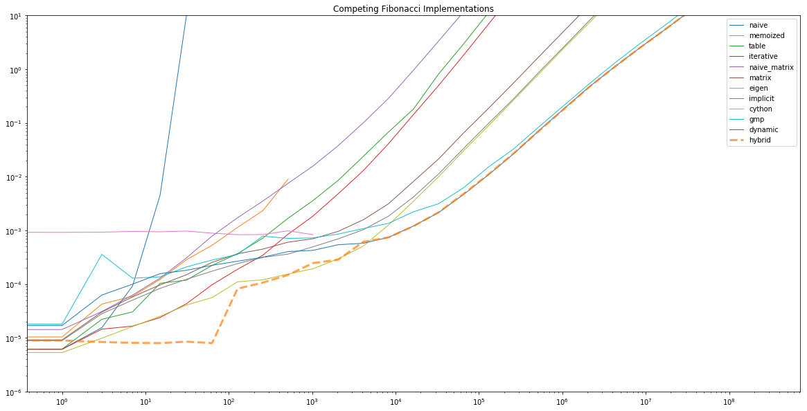
We can make a few observations:

• The naive implementation’s \(\mathcal{O}(2^n)\) performance hits a wall around 100, after which it’s no longer practical.
• The table based method actually runs out of memory before its runtime performance becomes a problem.
• The eigen_fib() implementation is basically constant time - until it starts overflowing once it can no longer represent its solution as a 64-bit floating point number.
• The best asymptotic performance is from the version using both GMP and the dynamic programming cache.
• By construction, the “hybrid” algorithm traces out lower bound - constant until 92, then hugs the Cython curve for a while, then switches to the dynamic GMP solution for large numbers.

Feynman Fuse Problem

We’ve made a lot of progress, and we’ve hit what I call a “fuse problem,” after this anecdote from Surely You’re Joking, Mr. Feynman!:

The problem was to design a machine like the other one - what they called a director - but this time I thought the problem was easier, because the gunner would be following behind in another machine at the same altitude. The gunner would set into my my machine his altitude and an estimate of his disance behind the other airplane. My machine would automatically tilt the gun up at the correct angle and set the fuse.

As director of this project, I would be making trips down to Aberdeen to get the firing tables. However, they already had some preliminary data and it turned out that the fuses they were going to use were not clock fuses, but powder-train fuses, which didn’t work at those altitudes - they fizzled out in the thin air.

I thought I only had to correct for the air resistance at different altitudes. Instead my job was to invent a machine that would make the shell explode at the right moment, when the fuse won’t burn!

I decided that was too hard for me and went back to Princeton.

Work on a problem long enough, and every problem is a fuse problem; that is to say, it becomes apparent that a fundamental shift in approach and a completely different skill set is necessary to make any further progress.

In our case, the problem is no longer to calculate Fibonacci numbers – the problem is now to find a way to multiply large integers together efficiently. As far as I can tell, GMP is already state-of-the-art when it comes to that, and tends to come out ahead on most benchmarks.

In fact, it’s recently come to my attention that GMP in fact has a dedicated Fibonacci benchmark. I can’t compete with that! So I think we’ve taken it as far as we can reasonably go.

Conclusion

When I started this project, I would not have believed that my laptop could calculate the millionth Fibonacci number in a fraction of a second. Certainly the first few algorithms we looked at couldn’t come close to that. But my surprise should come as no surprise.

New algorithms are being discovered all the time. When I graduated, quicksort was considered state-of-the-art. Since then, Timsort has supplanted it in a number of standard libraries such as Java’s. Some people believe improvements in algorithms are outpacing Moore’s law. Sometimes an algorithm comes along and just blows everything else out of the water, like John Platt’s Sequential Minimal Optimization. For a decade after that was invented, SVM’s were considered one of the best off-the-shelf classifiers, until even better algorithms came along. Even today, the best way to fit an ElasticNet model is to reduce it to an SVM and use a fast solver based on SMO.

New algorithms take even dedicated professionals by surprise. Kolmogorov – perhaps one of the greatest mathematicians of all time – actually stated the conjecture that multiplication was necessarily \(\mathcal{O}(n^2)\) in a lecture and a few weeks later his student Karatsuba showed how a few simple additions and subtractions would allow three multiplications to do the work of four, decreasing the bound to \(\mathcal{O}(n^{\log_2 3})\). So simple, yet until 1960 not one mathematician had ever thought of it. And yet it is this trick (and later more complicated versions in the same vein) that account for the almost magical speed of the GMP library. It’s also closely related to the same divide-and-conquer strategy for matrix multiplication that makes linear algebra libraries like OpenBLAS so fast.

The lower bounds on good algorithms can often seem impossible. It doesn’t sound possible to search a length \(n\) string for a substring of length \(m\) in less than \(\mathcal{O}(nm)\), but Rabin-Karp and other similar algorithms do it in \(\mathcal{O}(n+m)\) through the clever use of a rolling hash. It doesn’t sound possible to store and retrieve items in less than \(\mathcal{O}(\log n)\), but hash tables do it in amortized \(\mathcal{O}(1)\). Obviously, there’s absolutely no way to estimate the cardinality of the union of two possibly overlapping sets in less than \(\mathcal{O}(n \log n)\)… unless you use HyperLogLog. Bloom filters let you (for the price of a small change of a false positive but no chance of a false negative) test set membership while using only \(\mathcal{O}(\log n)\) space. How can it possibly do that? Hash functions again. In my own work, I frequently rely on sophisticated gradient descent algorithms to fit models that would take hours or days to fit on the same hardware if naive algorithms were used. All of these algorithms are somewhere between magical and impossible. Yet they all work, both in theory and practice.

As good as today’s hardware is, it’s often the algorithm that makes the impossible possible.

The code for today’s article is available as a Jupyter notebook if you’d like to hack on it. You will need to install GMP, its Python wrapper gmpy2, and Cython. I am sure there is another order of magnitude of performance to be found somewhere.