ML From Scratch, Part 3: Backpropagation

Representation

A complete description of typical fully-connected feed-forward \(L\)-layer neural network can be given in just four equations: two boundary conditions for the input and output layers, and two recurrence relationships for the connections between layers:

\[ \begin{split} a^{(0)} & = X \\ z^{(i)} & = W^{(i)} a^{(i-1)} + b^{(i)} \\ a^{(i)} & = \sigma(z^{(i)}) \\ \hat{y} & = a^{(L)} \end{split} \]

Here \(\sigma(x)\) is a sigmoid function, \(W^{(i)}\) are matrices of weights connecting layers, \(b^{(i)}\) are bias vectors, \(X\) is the given matrix of data with one row per observation and one column per feature, and the final activation \(a^{(L)}\) is also our prediction \(\hat{y}\).

(A brief aside about notation. A superscript inside of parentheses is a layer index; the parentheses are meant to distinguish it from an exponent. This notation is used so that ordinary subscripts can be used to refer to the individual elements of \(W\) and \(b\), for example, \(W_{jk}^{(i)}\) is the element in the \(j\)-th row of the \(k\)-th column of the weight matrix \(W^{(i)}\) for the \(i\)-th layer.)

All that’s really going on here is that we are alternating matrix multiplication with the element-wise application of a non-linear function, \(\sigma(x)\) in this case. Start with a signal \(X\). To propagate the signal through the network, multiply by a matrix \(W^{(1)}\); add in the bias, apply the activation function. Multiply by \(W^{(2)}\), add in the bias, apply the application function. Multiply by \(W^{(2)}\), add in the bias, apply the application function. Repeat until you reach the output layer.

Note that because of the restrictions on matrix multiplication, we can determine the number of rows and columns in each matrix \(W^{(i)}\) by noting that it much have a number of columns equal to the number of rows in \(W^{(i-1)}\). In particular that means \(W^{(1)}\) must have a number of columns equal to the number of features in the dataset \(X\), while \(W^{(L)}\) has only a single output row. We call this shared dimension the “number of nodes” in that layer of the neural network; you will see me use this terminology in the code below especially when initializing the network.

The parameters of the model are all the elements of every connection matrix \(W^{(i)}\) plus the elements of the bias vectors \(b^{(i)}\). In symbols:

\[ \Theta = (W^{(1)} ... W^{(L)}, b^{(1)} ... b^{(L)}) \]

A quick aside about the total number of parameters: Since every element of every weight matrix for every layer is a separate parameter, large neural networks tend to have a lot of parameters. This implies that neural nets have high VC dimension, which in turn implies that they tend to badly overfit unless the number of data points in the training set is a high multiple of the number of parameters. This is the fundamental reason why “deep neural networks” and “big data” go hand-in-hand.

Returning to the mathematics of our representation, let’s make this abstract recurrence relation concrete by showing explicit examples for small \(L\). For example, with zero hidden layers (\(L=1\)) a neural network reduces to the equation for logistic regression:

\[ \hat{y} =\sigma(W^{(1)} X + b^{(1)}) \]

If a zero-hidden-layer neural network is also trained with log-loss, both the model’s representation and fitted parameters will be exactly the same as logistic regression. We can view LR as a special case of neural nets or equivalently neural nets as a generalization of LR.

With one hidden layer (\(L=2\)) this expands to:

\[ \hat{y} =\sigma(W^{(2)} \sigma(W^{(1)} X + b^{(1)}) + b^{(2)}) \]

A logistic regression of logistic regressions, if you will. As the chain grows longer the same pattern is repeated:

\[ \hat{y} =\sigma(W^{(3)} \sigma(W^{(2)} \sigma(W^{(1)} X + b^{(1)}) + b^{(2)}) + b^{(3)}) \]

These examples are only included for the sake of concreteness. The recursive definitions will allow us to reason about a sequential neural network with any number of layers.

Fitting

To fit the model to data, we find the parameters which minimize loss: \(\hat{\Theta} = \text{argmin} \, J(\Theta;X)\). Just as with logistic regression we use binary cross-entropy (a.k.a. log-loss) which means our loss function \(J\) is given by:

\[ J = \frac{1}{N} \sum_i^N y_i \ln \hat{y}_i + (1-y_i) \ln (1-\hat{y}_i) \]

Note that we have introduced a \(1/N\) scale factor. We are free to do this because multiplying by a positive constant does not change the optimization problem. We do this so that the gradient will be an average over all the training examples and therefore will be invariant w.r.t. training set size. This turns out to be convenient because it means we will not need to change our learning rate when fitting larger or smaller datasets.

One condition which must be true at a local minima is that \(\nabla_\Theta J = 0\). That gives us the equations:

\[ \frac{\partial J}{\partial W^{(i)}} = 0, \frac{\partial J}{\partial b^{(i)}} = 0 \]

The notation used here is from matrix calculus, and we are taking partial derivatives with respect to a matrix (for \(W\)) or a vector (for \(b\).) The matrix cookbook may help with this notation.

Given the forward pass equations given above, we can easily calculate the partial derivatives for the individual components. For the derivation of \(\partial J / \partial a^{(L)}\) you can follow pretty much the same proof given in the previous article on logistic regression. For the others it is easy to verify from the above definitions that:

\[ \begin{split} \color{blue} \frac{\partial J}{\partial a^{(L)}} & \color{blue} = \frac{\partial J}{\partial \hat{y}} = \frac{1}{N} (y - \hat{y}) \\ \color{green} \frac{\partial a^{(i)}}{\partial z^{(i)}} & \color{green} = a^{(i)} \circ (1-a^{(i)}) \\ \color{green} \frac{\partial z^{(i)}}{\partial a^{(i-1)}} & \color{green} = W^{(i)} \\ \color{maroon} \frac{\partial z^{(i)}}{\partial W^{(i)}} & \color{maroon} = (a^{(i-1)})^T \end{split} \]

For the element-wise derivative of the sigmoid we use the slightly non-obvious fact that \(\sigma'(x) = \sigma(x) (1-\sigma(x))\) which we proved in Part 2. Also, take special note of the transpose on the last equation! This follows immediately from proposition (70) in the matrix cookbook but its importance is to introduce the inner product that sums over all the training examples; all the other terms have a number of rows equal to \(N\) (the number of training examples) and it is only in this last step that we reduce dimensionality to match that of \(W\). The practical implication is that the activations and backpropagated error terms we carry around during the calculation require an amount of memory proportional to \(N\). This is part of the reason why mini-batch gradient descent is a good idea when training neural networks.

From now on, we will be describing the equations for \(\nabla J\) in terms of partial derivatives - if you want to know how to actually calculate anything concretely, refer to these four equations.

To take a partial derivative of \(J\) with respect to any parameter in any layer we can use the chain rule. For \(W^{(L)}\) we have:

\[ \frac{\partial J}{\partial W^{(L)}} = \Bigg( \color{blue} \frac{\partial J}{\partial a^{(L)}} \color{black} \circ \color{green} \frac{\partial a^{(L)}}{\partial z^{(L)}} \color{black} \Bigg) \cdot \color{maroon} \frac{\partial z^{(L)}}{\partial W^{(L)}} \]

Where the dot product is defined as \(x \cdot y = (x^T y)^T\). This corresponds to the usual definition when \(x\) and \(y\) are vectors but is extended to matrices. You can think of it as summing over all the examples in the training set. This notation isn’t 100% standard but I’m going to use it anyway because it lets us write out the chain rule in the usual left-to-right manner.

Next, let’s do \(W^{(L-1)}\):

\[ \frac{\partial J}{\partial W^{(L-1)}} = \Bigg( \underbrace{ \color{blue} \frac{\partial J}{\partial a^{(L)}} \color{black} \circ \color{green} \frac{\partial a^{(L)}}{\partial z^{(L)}} }_{Old} \color{green} \circ \color{black} \underbrace{ \color{green} \frac{\partial z^{(L)}}{\partial a^{(L-1)}} \circ \frac{\partial a^{(L-1)}}{\partial z^{(L-1)}} }_{\text{New}} \color{black} \Bigg) \cdot \color{maroon} \frac{\partial z^{(L-1)}}{\partial W^{(L-1)}} \]

Then \(W^{(L-2)}\):

\[ \frac{\partial J}{\partial W^{(L-2)}} = \Bigg( \underbrace{ \color{blue} \frac{\partial J}{\partial a^{(L)}} \color{black} \circ \color{green} \frac{\partial a^{(L)}}{\partial z^{(L)}} \circ \frac{\partial z^{(L)}}{\partial a^{(L-1)}} \circ \frac{\partial a^{(L-1)}}{\partial z^{(L-1)}} }_{Old} \color{green} \circ \color{black} \underbrace{ \color{green} \frac{\partial z^{(L-1)}}{\partial a^{(L-2)}} \circ \frac{\partial a^{(L-2)}}{\partial z^{(L-2)}} \color{black} }_{New} \Bigg) \cdot \color{maroon} \frac{\partial z^{(L-2)}}{\partial W^{(L-2)}} \]

By now you should be starting to see a pattern emerge: as we go back layer by layer, the left-most part of the equation (blue and green) for layer \(i\) is always the same as the blue and green part from layer \(i+1\) plus two more new green factors, and capped off by the final maroon factor.

Think of it like a snake: We always start with the (blue) derivative of our loss function with respect to the prediction. This only happens once so stays at the “head” of the equation. At the (maroon) “tail”, we always take a derivative with respect to the parameters of interest. And in between we between we have a growing (green) “body” of partial derivatives. To capture this insight in symbols, let’s introduce a new recurrence relation:

\[ \begin{split} \color{purple} \delta^{(L)} & = \color{blue} \frac{\partial J}{\partial a^{(L)}} \color{black} \circ \color{green} \frac{\partial a^{(L)}}{\partial z^{(L)}} \color{black} \\ \color{purple} \delta^{(i-1)} & = \color{purple} \delta^{(i)} \color{black} \circ \Bigg( \color{green} \frac{\partial z^{(i)}}{\partial a^{(i-1)}} \circ \frac{\partial a^{(i-1)}}{\partial z^{(i-1)}} \color{black} \Bigg) \\ \frac{\partial J}{\partial W^{(i)}} & = \color{purple} \delta^{(i)} \color{black} \circ \color{maroon} \frac{\partial z^{(L-2)}}{\partial W^{(L-2)}} \end{split} \]

It should also be clear that we can implement this iteratively if we start at layer \(L\) and work backwards: If we save the result of the blue and green parts from layer \(i\), we can add on another pair of green partial derivates to grow the “body” and quickly compute layer \(i-1\). Note also that in order to calculate \(\color{green} \partial a / \partial z\) we need to know the activations which are most easily obtained by first performing a forward pass and remembering the activations for use in the backwards pass.

Finally, I’d like to point out that the justification for introducing the (technically extraneous) concept of \(z\) is found in how absolutely obvious and clear it makes the separate steps of the forward and backwards pass. If we had to take \(\partial a^{(i)} / \partial a^{(i-1)}\) directly without going through \(z\) we would have to think about a non-linear function of a matrix all at once; with \(z\) we’re able to view it as the element-wise application of a non-linear function (which is Calculus 101) and the partial derivative of a linear expression with respect to a matrix (which is Matrix Calculus 101; see the Cookbook).

Implementation

The above equations are straight-forward to turn into working code. The only wrinkle is that while above we represented the bias as separate vectors \(b^{(i)}\), in the implementation we will instead implement the bias by assuring that the matrix \(X\) and all intermediate activations \(a^{(i)}\) have a constant 1 in their first column. Thus, in the Python implementation the first column of each \(W^{(i)}\) plays the role of the bias vector. This simplifies the code in some ways but complicates it in others; pay attention to where we are stacking the bias node (or removing it during the backwards pass) and the apparent off-by-one “mismatch” in matrix dimensions this introduces.

import numpy as np

def sigmoid(z):
    return 1 / ( 1 + np.exp(-z) )

class NeuralNetwork:
    def __init__(self, 
                 n_hidden=(100,),
                 learning_rate=1.0,
                 max_iter=10,
                 threshold=0.5):
        # a list containing the number of nodes in 
        # each hidden layer.
        self.n_hidden = n_hidden
        
        # the input layer, output layer, and hidden layers.
        self.n_layers = len(n_hidden) + 2
        
        # gradient descent parameters
        self.learning_rate = float(learning_rate)
        self.max_iter = int(max_iter)
        self.threshold = float(threshold)

Initializing a neural network correctly turns out to be very important. If we punt and simply initialize all weights to a constant, the network will flat out not work to any meaningful degree. That’s new; linear regression and logistic regression certainly didn’t exhibit that behavior. Why is this the case? Well, if all the weights in a given layer are exactly the same at iteration \(i\), then the backpropagated error for each node with be exactly the same, so the gradient descent update will be exactly the same, so all the weights in the layer at iteration \(i+1\) will be exactly the same. By induction, this will be true for all iterations. Because all the weights of given layer are constrained to be the same, we effectively have only one free parameter! Our model will never learn the complex representations we want it to. Luckily, this critical point is almost surely unstable, so we can break symmetry by simply initializing the weights slightly differently. There are a couple popular ways to do this (one due to Glorot and Bengio and another due to He et al.) but since I don’t claim to understand either of those in great detail, to conform with the constraints of the “from scratch” project I’ll do something I do understand and just randomly initialize them randomly distributed by \(\mathcal{N}(0, 0.1^2)\). That suffices to break symmetry.

    def _random_initialization(self):
        # a small amount of randomization is necessary to
        # break symmetry; otherwise all hidden layers would
        # get updated in lockstep.
        if not self.n_hidden:
            layer_sizes = [ (self.n_output, self.n_input+1) ]
        else:
            layer_sizes = [ (self.n_hidden[0], self.n_input+1) ]
            previous_size = self.n_hidden[0]

            for size in self.n_hidden[1:]:
                layer_sizes.append( (size, previous_size+1) )
                previous_size = size

            layer_sizes.append( (self.n_output, previous_size+1) )
        
        self.layers = [
            [np.random.normal(0, 0.1, size=layer_size), sigmoid]
            for layer_size in layer_sizes
        ]

Fitting is straight-forward: for every iteration we do one forward-pass to calculated activations, then one backwards pass to calculated gradients and update all the weights. You may notice that we’ve reverted to batch gradient descent; today’s focus is on the representation of neural networks and the backpropagation algorithm, so we’ll keep everything else as simple as possible. You can read about more sophisticated gradient descent methods in the previous article in this series.

    def fit(self, X, y):
        self.n_input = X.shape[1]        
        self.n_output = 1
        y = np.atleast_2d(y).T
        self._random_initialization()
        
        # fitting iterations
        for iteration in range(self.max_iter):
            self.forward_propagation(X)
            self.back_propagation(y)
        
    def predict(self, X):
        y_class_probabilities = self.predict_proba(X)
        return np.where(y_class_probabilities[:,0] < self.threshold, 0, 1)
    
    def predict_proba(self, X):
        self.forward_propagation(X)
        return self._activations[-1]

The forward pass follows our above recursive definition of the neural network very closely. We initialize activation with the given predictors \(a^{(0)} = X\) then iteratively compute \(a^{(1)}\), \(a^{(2)}\) until we reach \(a^{(L)} = \hat{y}\).

    def forward_propagation(self, X):
        # we will store the activations calculated at each layer
        # because these can be used to efficiently calculate
        # gradients during backpropagation.
        self._activations = []
        
        # initialize the activation with the given data
        activation = X  
        
        # forward propagation through all layers
        for W, activation_function in self.layers:
            bias = np.ones( (activation.shape[0], 1) )
            activation = np.hstack([bias, activation])
            self._activations.append(activation)
            activation = activation_function(activation @ W.T)    
        
        # the final activation layer does not have a bias node added.
        self._activations.append(activation)

For the backwards pass, we use error to mean \(\partial J / \partial z_i\) and delta to mean \(\partial J / \partial W_i\). We use the recurrence relations we derived from the chain rule to iteratively calculate the update for each layer counting down from \(L\) to \(1\).

    def back_propagation(self, y):
        # this function relies on self._activations calculated
        # by self.forward_propagation()

        N = y.shape[0]
        
        # the final prediction is simply activation of the final layer.
        y_hat = self._activations[-1]
        
        # this first error term is based on the gradient of the loss function:
        # log-loss in our case. Subsequently, error terms will be based on the 
        # gradient of the sigmoid function. 
        error = y_hat - y
        
        # we can see where the backpropagation algorithm gets its name: we
        # start at the last layer and work backwards, propagating the error
        # term from each layer to the previous one.
        for layer in range(self.n_layers-2, -1, -1):
            # calculate the update (delta) for the weight matrix
            a = self._activations[layer]
            
            delta = (error.T @ a) / N
            
            # every layer except the output layer has a bias node added.
            if layer != self.n_layers-2:
                delta = delta[1:, :]
            
            # propogate the error term back to the previous layer
            W = self.layers[layer][0]
            if layer > 0:
                
                # every layer except the output layer has a bias node added.
                if layer != self.n_layers-2:
                    error = error[:, 1:]
                    
                # the a(1-a) is the gradient of the sigmoid function.
                error = (error @ W) * (a * (1-a))
            
            # update weights
            W -= self.learning_rate * delta

Testing

Real world data are messy. Instead of shopping around for a toy data set which exhibits all the properties we want, we’ll cook up an idealized data set that is designed to only be solvable by a non-linear classifier.

from sklearn import datasets

X_full, y_full = datasets.make_classification(
    n_samples=5000, n_features=20,
    n_informative=15,
    n_redundant=3,
    n_repeated=0,
    n_classes=2,
    flip_y=0.05,
    class_sep=1.0,
    shuffle=True,
    random_state=42)

# 80/20 train/test split. 
train_test_split = int(0.8 * len(y_full))
X_train = X_full[:train_test_split, :]
y_train = y_full[:train_test_split]
X_test = X_full[train_test_split:, :]
y_test = y_full[train_test_split:]

This synthetic dataset has 4,000 examples in the training set and 1,000 in the test set. There are two classes with equal prevalence. There are 20 features, but only about half of these have non-zero mutual information with the class. 5% of examples simply have their class flipped, so the Bayes rate will be less than 0.05; in other words, the ceiling for accuracy is less than 95%. Each vertex is assigned to one class or the other and then data is sampled from a standard multivariate Gaussian distribution centered at each vertex. In particular, because vertices are only one standard deviation away from each other these distributions will overlap a good deal and further reduce the Bayes rate. The problem is highly non-linear and classifiers with linear decision boundaries will struggle; however it not at all pathological and a good non-linear classifier should be able to achieve something quite close to the Bayes rate.

When we fit a model, the number of hidden layers and the node of nodes in each layer is a hyperparameter. For example, two hidden layers with 20 nodes in the first layer and 5 in the second would be [20, 5].

nn = NeuralNetwork(n_hidden=[8, 3], max_iter=2000)
nn.fit(X_train, y_train)
y_hat = nn.predict(X_train)
p_hat = nn.predict_proba(X_train)
np.mean(y_train == y_hat)

If we have no hidden layers at all then our neural network reduces to logistic regression. In particular that means it can only learn an linear decision boundary. How well does that do on the synthetic dataset we cooked up?

nn = NeuralNetwork(n_hidden=[], max_iter=2000)
nn.fit(X_train, y_train)
y_hat = nn.predict(X_train)
p_hat = nn.predict_proba(X_train)
y_test_hat = nn.predict(X_test)
p_test_hat = nn.predict_proba(X_test)
np.mean(y_train == y_hat), np.mean(y_test == y_test_hat)

(0.71924999999999994, 0.71699999999999997)

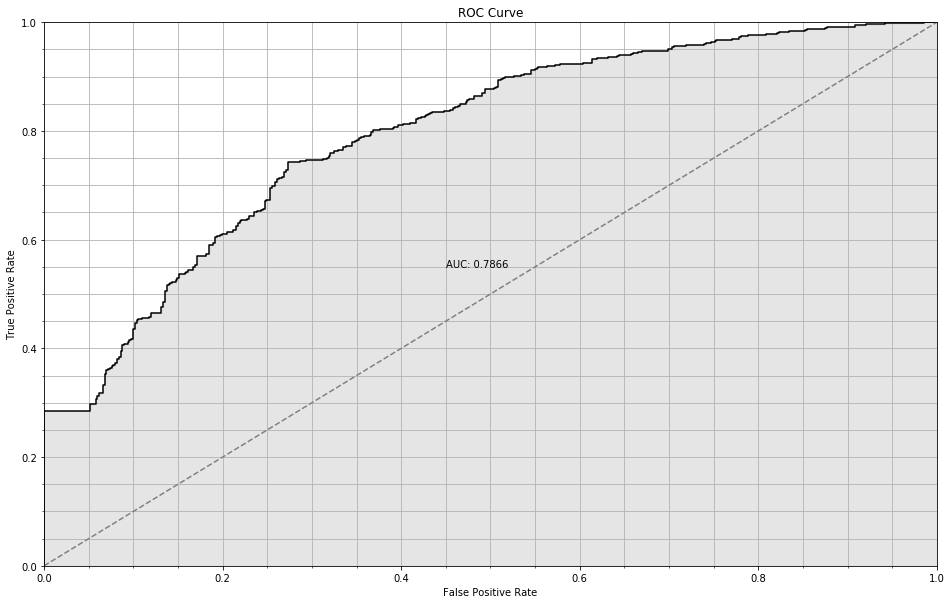
Not so hot: about 72% accuracy, and an AUC of 0.7866. That’s pretty far away from the Bayes rate we estimated above; therefore we are probably underfitting.

from sklearn.metrics import roc_curve, roc_auc_score
from matplotlib import pyplot as plt
%matplotlib inline

fpr, tpr, threshold = roc_curve(y_test, p_test_hat)
plt.figure(figsize=(16,10))
plt.step(fpr, tpr, color='black')
plt.fill_between(fpr, tpr, step="pre", color='gray', alpha=0.2)
plt.xlabel("False Positive Rate")
plt.ylabel("True Positive Rate")
plt.title("ROC Curve")
plt.plot([0,1], [0,1], linestyle='--', color='gray')
plt.text(0.45, 0.55, 'AUC: {:.4f}'.format(roc_auc_score(y_test, p_test_hat)))
plt.minorticks_on()
plt.grid(True, which='both')
plt.axis([0, 1, 0, 1])

On the other extreme, after trying a couple of hyperparameters, I found that [8,3] worked reasonably well.

nn = NeuralNetwork(n_hidden=[8, 3], max_iter=2000)

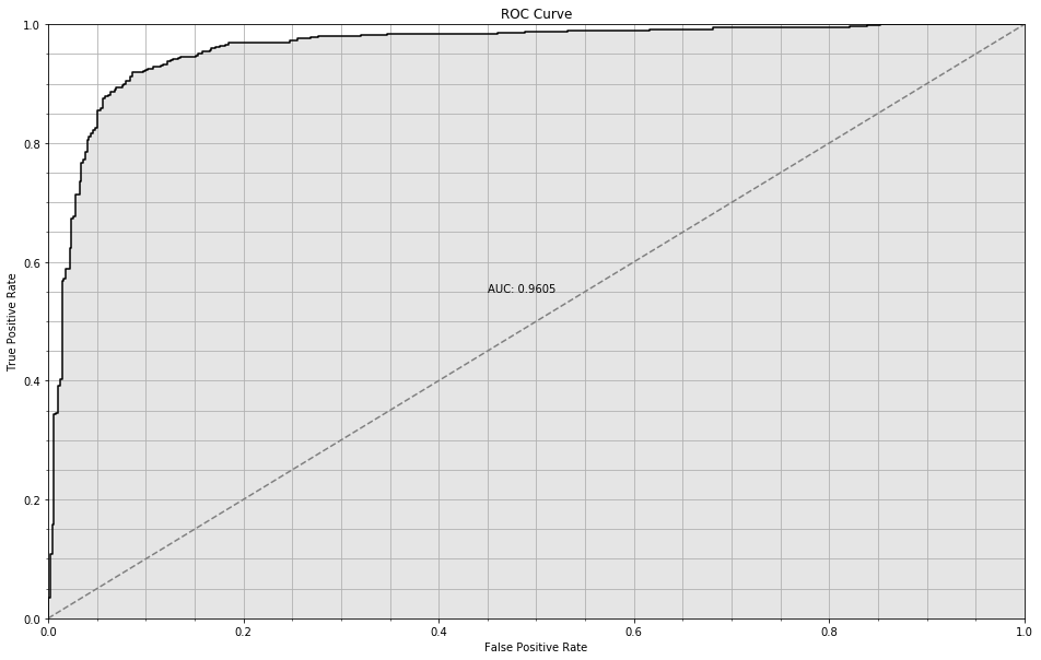
The [8, 3] model achieves 0.96 AUC and 95% accuracy on the training set and 91% accuracy on the test set. This is enormously better than what was possible with a linear decision boundary.

This new model has two hidden layers of 8 nodes and 3 nodes respectively; all layers are fully connected, so there’s a \(9 \times 3\) matrix with 27 parameters connecting them, plus the \(4 \times 1\) connecting to the output node and the \(21 \times 8\) matrix connecting to the input layer, making for 199 parameters in all. Therefore it’s no surprise that its able to fit the training set much more closely, but it is very pleasant surprise that this means its test set performance is also much improved!

We can get a better intuition for the relationship between the complexity of our neural network and performance by plotting test set AUC as a function of the number of node used:

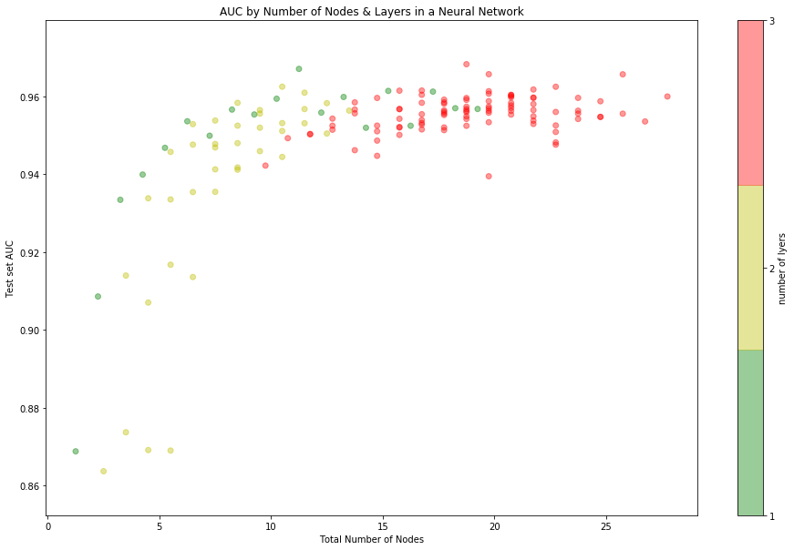
There’s a clear elbow in the graph around 10 nodes. Below that, the model makes steady gain in performance as more nodes to the model and its representation becomes better equipped to deal with the non-linearity of the true distribution. Above 10 nodes, making the model more complex is not able to further reduce generalization error; This suggests that the [8,3] model we found earlier is about as good as we can do.

As a rule of thumb, the more data available for training, the more features, and the more non-linear/interaction effects in the true population, the more that elbow gets pushed to the right; in other words, The model doesn’t start to overfit until much later. For best results, the complexity of the neural network should mirror the complexity of the underlying problem. One advantage of neural networks is that they give us an easy way to make the model arbitrarily “smarter” simply by adding more layers and more neurons. In fact, not only can we simply throw more neurons and layers at a problem, we also have a wide variety of specialized layers like CNNs which can make a neural network more suited to a particular problem. The neural network is a very “modular” learning algorithm in this sense and the flexibility means in can be adapted to a wide variety of problems.

Unfortunately, the strategy of bigger, smarter neural networks is only really viable when we have a ton of training data. Smart neural networks trained on small datasets overfit horribly long before they learn to generalize. Neural networks don’t solve the bias-variance trade-off for us, and they certainly aren’t a free lunch. But they do provide a framework for creating models with low bias even on very large and difficult problems… then it’s our job to keep the variance in check.

Conclusion

That was backpropagation from scratch, our first look at neural networks. We saw how a sequential feed-forward network could be represented as alternating linear and non-linear transforms. We saw how to use the chain rule to calculate the gradient of the loss function with respect to any parameter in any layer of model, and how to calculate these gradients efficiently using the backpropagation algorithm. We demonstrated that a neural network could solve non-linear classification problems that logistic regression struggled with. And finally we saw how we could tune the number of layers and nodes in the neural network to take advantage of large datasets.

The specific neural network presented in this article is incredibly simple relative to the neural networks used to solve real world problems. For example, we haven’t yet talked about the vanishing gradient problem and how it can be solved with rectified linear units or batch normalization, how convolutional layers or pooling can help when the data have a natural spatial structure, how residual networks wire layers together as acyclic digraphs, how recurrent neural networks use short-term memory to handle arbitrary sequences of inputs, or a thousand other topics. Yet today, the state-of-the-art algorithm used to train all of these varied species of neural networks is backpropagation, exactly as presented here.

In practice, it isn’t usually necessary to actually do the calculus by hand. Modern machine learning frameworks like Tensorflow or PyTorch prominently feature automatic differentiation as a core capability. The chain rule is straightforward to apply mechanically - the hard part is keeping track of all those indices! So it makes sense to have software handle it.

In the next installment of the Machine Learning From Scratch series (coming soon!) we will change tact and look at a completely different approach to non-linear classification: decision trees and the recursive partition algorithm. We will see how these two apparently diametrically opposed approaches can both be viewed as examples of adaptive basis functions, and how this point-of-view unifies disparate topics in machine learning.