ML From Scratch, Part 4: Decision Trees

Gini Impurity and Information Gain

The first thing we need to pin down is what we mean by “better” and “less balanced.” There are two competing definitions; I’ll describe both and then pick one to use for the implementation.

The first, Gini impurity, is defined as the probability that a randomly chosen element will be misclassified if we randomly choose a prediction from the distribution of classes itself.

\[ I_G(\mathbf{p}) = \sum_{i} \mathbf{p}_i \sum_{j \neq i} \mathbf{p}_j \]

In the binary case, we usually simplify the notation and refer to \(\mathbf{p}_1 = p\) and \(\mathbf{p}_2 = 1-p\), yielding this much simpler expression:

\[ \begin{align} I_G(p) & = p(1-p) + (1-p)p = 2p(1-p) \\ \Delta I_G & = I_{\text{parent}} - p_{\text{left}} I_{\text{left}} - p_{\text{right}} I_{\text{right}} \end{align} \]

Interestingly enough, this is not how we will actually make predictions – we will in fact always choose the most likely class.

An example can make this much more concrete. Suppose we have 100 observations with two balanced classes; exactly 50 each. If our decision tree consists of only a root, we have to make the constant prediction 0.5 for all possible inputs, so our Gini impurity is 0.5. But once we split the root node, we’ll have two leafs, and these will unbalanced classes, say 40/10 and 10/40. The Gini impurity of these two nodes is \(2 \times .2 \times .8 = .32\). When we make a prediction, every input will be assigned to one of these two leaf nodes. If it ends up in the left node, we will predict class 0 and be right 80% of the time. If it ends up in the right node, we will predict class 1 and still be right 80% of the time. Accuracy has improved from 50% to 80%. However, if instead of always choosing the most likely class, we instead made our predictions randomly, sampling from a Bernoulli distribution with parameter \(p = 0.2\) for the left node and \(p = 0.8\) for the right node, we would be right 68% of time. This is the converse of Gini impurity. It’s a trivial theorem that we can always minimize error and maximum accuracy by choosing the most likely class, so that’s what we’ll use for decision rule. But Gini impurity does a better job of capturing / representing how much we’ve learned, so that’s what we’ll use to train.

Second, there’s a competing metric called entropy which is often used instead of Gini impurity. There’s a long derivation where entropy is defined as the log of the probability mass function of a multinomial distribution, information is defined as the opposite of entropy, and information gain is defined as the difference between the entropy of the parent node and the weighted sum of the entropies of all child nodes, but long story short, for the simple case with just two classes the formula looks like this:

\[ \begin{align} H & = -p \ln p - (1-p) \ln (1-p) \\ \Delta H & = H_{\text{parent}} - p_{\text{left}} H_{\text{left}} - p_{\text{right}} H_{\text{right}} \end{align} \]

Both functions are symmetric about the line \(x = 0.5\) and both are strongly concave. This turns out to be very important, because it means it’s always possible to choose a good cut point. Other metrics, such as accuracy, don’t have this property but instead give the exact same “goodness” score for many different candidate splits.

Modulo a scaling factor, entropy has almost the same shape as the Gini impurity:

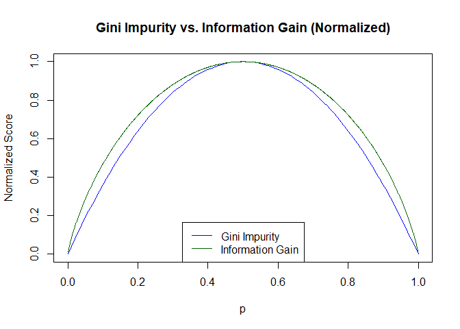
These small differences in shape don’t usually result in different decisions about which feature to choose or where to make the split, so decision trees trained on one or the other will often be identical and usually have identical performance. We will use Gini impurity because it is slightly cheaper to calculate a square than a log.

Finding The Best Cut Point

At each stage, we have two decisions to make: which feature to use for the cut, and the exact value to cut out. Each rule is of the form

\[ X_i \leq C \]

While it would be possible to simply brute force our way through all possible cut points, calculating Gini impurity from scratch each and every time, this is hugely slower than a more efficient (but slightly harder to understand) vectorized algorithm. We, of course, will choose the path of most resistance and highest performance.

def best_split_point(X, y, column):
    # sorting y by the values of X makes
    # it almost trivial to count classes for
    # above and below any given candidate split point. 
    ordering = np.argsort(X[:,column])
    classes = y[ordering]

    # these vectors tell us how many of each
    # class are present "below" (to the left)
    # of any given candidate split point. 
    class_0_below = (classes == 0).cumsum()
    class_1_below = (classes == 1).cumsum()
    
    # Subtracting the cummulative sum from the total
    # gives us the reversed cummulative sum. These
    # are how many of each class are above (to the
    # right) of any given candidate split point.
    #
    # Because class_0_below is a cummulative sum
    # the last value in the array is the total sum.
    # That means we don't need to make another pass
    # through the array just to get the total; we can
    # just grab the last element. 
    class_0_above = class_0_below[-1] - class_0_below
    class_1_above = class_1_below[-1] - class_1_below
    
    # below_total = class_0_below + class_1_below
    below_total = np.arange(1, len(y)+1)
    # above_total = class_0_above + class_1_above
    above_total = np.arange(len(y)-1, -1, -1)

    # we can now calculate Gini impurity in a single
    # vectorized operation. The naive formula would be:
    #
    #     (class_1_below/below_total)*(class_0_below/below_total)
    # 
    # however, divisions are expensive and we can get this down
    # to only one division if we combine the denominator term.
    gini = class_1_below * class_0_below / (below_total ** 2) + \
           class_1_above * class_0_above / (above_total ** 2)

    gini[np.isnan(gini)] = 1
    
    # we need to reverse the above sorting to
    # get the rule into the form C_n < split_value. 
    best_split_rank = np.argmin(gini)
    best_split_gini = gini[best_split_rank]
    best_split_index = np.argwhere(ordering == best_split_rank).item(0)
    best_split_value = X[best_split_index, column]
    
    return best_split_gini, best_split_value, column

Building the Tree

The fundamental building block of a tree is the “Node.” In our implementation, every node starts life as a leaf node, but when it the .split() method is invoked, it mutates into a branch node with two new leaf nodes underneath. The split is made by calculating the optimal split point for each feature, then choosing the feature and split point which minimizes Gini impurity. This continues recursively for both children until a node is perfectly pure or the maximum depth parameter is reached.

class Node:
    def __init__(self, X, y):
        self.X = X
        self.y = y
        self.is_leaf = True
        self.column = None
        self.split_point = None
        self.children = None
    
    def is_pure(self):
        p = self.probabilities()
        if p[0] == 1 or p[1] == 1:
            return True
        return False

    def split(self, depth=0):
        X, y = self.X, self.y
        if self.is_leaf and not self.is_pure():
            splits = [ best_split_point(X, y, column) for column in range(X.shape[1]) ]
            splits.sort()
            gini, split_point, column = splits[0]
            self.is_leaf = False
            self.column = column
            self.split_point = split_point
            
            below = X[:,column] <= split_point
            above = X[:,column] > split_point 
            
            self.children = [
                Node(X[below], y[below]),
                Node(X[above], y[above])
            ]
            
            if depth:
                for child in self.children:
                    child.split(depth-1)

We will will also make our Node class responsible for predicting probabilities (but not classes.) To obtain predictions from a branch node, we simply use the learned rule to decide whether to descend to the left or right child. When we reach a leaf, we can return a probability based on the proportion of classes in the leaf.

def probabilities(self):
    return np.array([
        np.mean(self.y == 0),
        np.mean(self.y == 1),
    ])

def predict_proba(self, row):
    if self.is_leaf:
        return self.probabilities()
    else:
        if row[self.column] <= self.split_point:
            return self.children[0].predict_proba(row)
        else:
            return self.children[1].predict_proba(row)

This prediction step can also be vectorized by applying a separate vectorized filter for each leaf node. However, in a tree of depth \(k\), this requires calculating \(2^k\) separate filters, each comprised of the logical AND of \(k\) separate comparisons. This is not usually faster than just applying the rules row-by-row.

Interface

The above Node class can be used directly to fit models but as we’ve done elsewhere in the series we give our model a user-friendly, scikit-learn style interface. The class keeps track of only a single “root” Node, and relies on that root node’s recursive .split() and .predict_proba() methods to reach deeper nodes.

class DecisionTreeClassifier:
    def __init__(self, max_depth=3):
        self.max_depth = int(max_depth)
        self.root = None
        
    def fit(self, X, y):
        self.root = Node(X, y)
        self.root.split(self.max_depth)
        
    def predict_proba(self, X):
        results = []
        for row in X:
            p = self.root.predict_proba(row)
            results += [p]
        return np.array(results)
            
    def predict(self, X):
        return (self.predict_proba(X)[:, 1] > 0.5).astype(int)

Testing

The scikit-learn breast cancer dataset is a good choice for testing decision trees because it is high dimensional and highly non-linear.

# a small classification data set with 30 to get with. 
breast_cancer = load_breast_cancer()
X = breast_cancer.data
y = breast_cancer.target

model = DecisionTreeClassifier(max_depth=4)
model.fit(X, y)
y_hat = model.predict(X)
p_hat = model.predict_proba(X)[:,1]

The models out-of-the-box (by “out-of-the-box” I mean, “without need for hyper-parameter selection via cross-validation”) performance is quite good:

print(confusion_matrix(y, y_hat))
print('Accuracy:', accuracy_score(y, y_hat))

                 True Class
                    P     N
 Predicted     P  193    19
 Class         N   18   339

 Accuracy: 0.9349736379613357

This confusion matrix and accuracy are only part of the story - in particular, they are performance we see if we choose to define a positive test result as \(p > 0.5\). We can get a broader view the models performance over a range of possible thresholds with an ROC curve:

ROC Curve

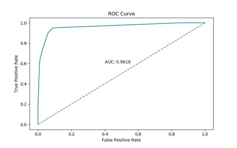
An AUC of .96 is pretty respectable.

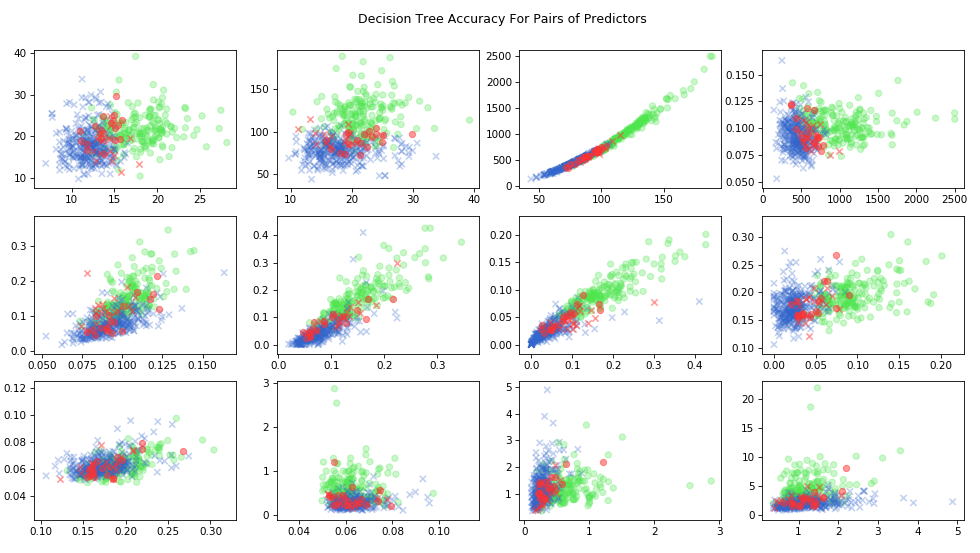
We can also look at the results as a function of the predictor variable \(X\). Since there are 30 separate features, we will just look at a representative sample. For each pair of predictor variables, we’ll plot true positives in green, true negatives in blue, and misses in red.

plt.figure(figsize=(16,30))
markers = ['o', 'x']
red = (1, 0.2, 0.2, 0.5)
green = (0.3, 0.9, 0.3, 0.3)
blue = (0.2, 0.4, 0.8, 0.3)

for i in range(28):
    plt.subplot(7, 4, i+1)
    for cls in [0, 1]:
        mask = (y == cls) & (y == y_hat)
        plt.scatter(
            x=X[mask,i], 
            y=X[mask,i+1], 
            c=[blue if positive else green for positive in y[mask]],
            marker=markers[cls]
        )
        mask = (y == cls) & (y != y_hat)
        plt.scatter(
            x=X[mask,i], 
            y=X[mask,i+1], 
            c=red,
            marker=markers[cls],
            zorder=10
        )

Decision Tree Pairs

A simple text-based visualization of our tree can be done by adding a formatted() method to the Node() class:

def formatted(self, indent=0):
    if self.is_leaf:
        s = "Leaf({p[0]:.3f}, {p[1]:.3f})".format(p=self.probabilities())
    else:
        s = "Branch(X{column} <= {split_point})\n{left}\n{right}".format(
            column=self.column, 
            split_point=self.split_point,
            left=self.children[0].formatted(indent+1),
            right=self.children[1].formatted(indent+1))
        
    return "    " * indent + s

def __str__(self):
    return self.formatted()

def __repr__(self):
    return str(self)

The breast cancer decision tree has the following structure, where greater indentation corresponds to greater depth in the tree.

Branch(X22 <= 89.04)
    Branch(X6 <= 0.0)
        Leaf(0.000, 1.000)
        Branch(X16 <= 0.0009737)
            Leaf(0.000, 1.000)
            Branch(X16 <= 0.001184)
                Leaf(0.000, 1.000)
                Branch(X19 <= 0.004651)
                    Leaf(0.013, 0.987)
                    Leaf(0.000, 1.000)
    Branch(X22 <= 96.42)
        Branch(X6 <= 0.004559)
            Leaf(0.000, 1.000)
            Branch(X6 <= 0.01063)
                Leaf(0.000, 1.000)
                Branch(X9 <= 0.05913)
                    Leaf(0.059, 0.941)
                    Leaf(0.086, 0.914)
        Branch(X26 <= 0.3169)
            Branch(X22 <= 117.7)
                Branch(X14 <= 0.006133)
                    Leaf(0.109, 0.891)
                    Leaf(0.273, 0.727)
                Branch(X19 <= 0.002581)
                    Leaf(0.875, 0.125)
                    Leaf(1.000, 0.000)
            Branch(X20 <= 27.32)
                Branch(X20 <= 27.32)
                    Leaf(0.902, 0.098)
                    Leaf(0.000, 1.000)
                Leaf(1.000, 0.000)

Note that several paths down the tree lead to immediately to large, totally pure leaf nodes. That’s because in this particular dataset, there are large regions of the input space which can be unambiguously classified. However, as we get closer to the true decision boundary, the predictions become more probabilistic, and we may only be able to say that perhaps 87.5% of cases will be negative.

Conclusion

Today we saw a simple and intuitive algorithm tackle a difficult, highly non-linear problem and achieve surprisingly good out-of-the-box performance after only a few seconds of training time.

Unfortunately, decision trees are exponentially data-hungry: to further improve performance (without overfitting) we would need to add more nodes to our model, but each layer that we add more than doubles the amount of data we need before our leaves have too few data points to reliably split. On this small dataset, we can’t go beyond three or four layers.

Another issue is that the decision boundary of a decision tree is a series of orthogonal, axis-aligned hyperplanes. This is rarely a well-motivated boundary – the real world contains diagonals and curves! – and as such would not be expected to generalize well. With a very deep tree, a diagonal or curved boundary can be approximated, yet this can require a large amount of data close to the decision boundary. However, decision trees can do very well when given discrete features.

The problems with decision trees stem from the fact they “believe” that the left hand should not know what the right hand is doing – yet in many cases it would make sense to pick the same decision rule for both sides of a decision tree. In fact, while decision trees are occasionally used directly on datasets, their real importance is in their use as the main ingredient in two state-of-the-art ML algorithms that do exactly this! Both random forest and extreme gradient boosting are examples of additive models built by combining different trees together. This allows them to have many different partially overlapping regions. We will look at these models in a future article; for now, let me just mention that there are some good arguments that suggest that any set of weak learners can be turned into a strong leaner when combined together in the right way, and these practical algorithms appear to “work” because of these deeper theorems.