
ML From Scratch V: Gaussian Mixture Models
Consider the following motivating dataset:
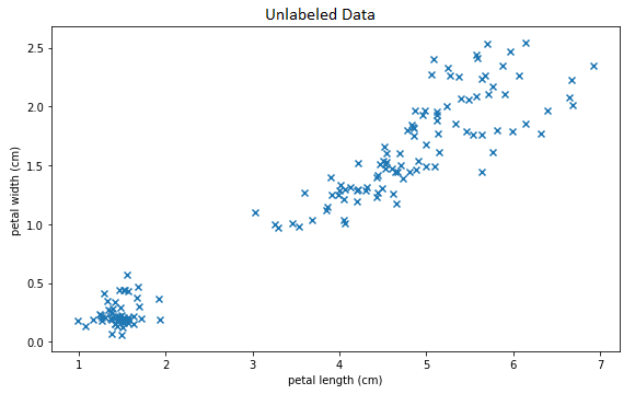
It is apparent that these data have some kind of structure; which is to say, they certainly are not drawn from a uniform or other simple distribution. In particular, there is at least one cluster of data in the lower right which is clearly separate from the rest. The question is: is it possible for a machine learning algorithm to automatically discover and model these kinds of structures without human assistance?
Every model we’ve look at so far has assumed that we have a clear definition of the thing we are trying to predict and that we already know the correct answer for every example in the training set. A problem of the form “just find me some kind interesting relationships or structure, any will do” does not fit into this framework because no “true” labels are known in advance. More formally: every problem so far has been a “supervised” learning problem, where the training set consists of labeled pairs $(X, Y)$ and the task was to predict $Y$ from $X$. The problem of discovering interesting structure or relationships from unlabeled examples $X$ is called the “unsupervised” learning problem, and calls for a different set of techniques and algorithms entirely.
Types of Unsupervised Learning
There are two broad approaches to unsupervised learning: dimensionality reduction and cluster analysis.
In dimensionality reduction we seek a function $f : \mathbb{R}^a \mapsto \mathbb{R}^b$ where $a$ is the dimension of the original data $\mathbf{X}$ and $b$ is usually much smaller than $a$. The classic example of a dimensionality reduction algorithm is PCA but there are many others, including non-linear techniques like t-SNE, topic models like LDA, and most examples of representation learning such as Word2Vec. The basic idea is that by reducing to a lower dimensional space we somehow capture the essential characteristics of each data point while getting rid of noise, multicollinearity, and non-essential features. Furthermore, it should be possible to approximately reconstruct the original data point in the original $a$-dimensional space from just its compressed $b$-dimensional representation with minimal loss. Depending on the specific technique used, the lower dimensional space may also be designed to have desirable properties like an isotropic/spherical covariance matrix or a meaningful distance function where data points that a human would agree are “similar” are close together. We will return to dimensionality reduction in some future article.
The second approach to unsupervised learning is called clustering and is characterized by seeking a function $f : \mathbb{R}^a \mapsto {1,2, …, k}$ which maps each data point to exactly one of $k$ possible classes. The classic example of a clustering algorithm is $k$-means. Reducing rich, multivariate data to a small finite number of possibilities seems extreme, but for that same reason it can be extremely clarifying as well. In this article we will implement on particular clustering model called the Gaussian mixture model, or just GMM for short.
Gaussian Mixture Models
The Gaussian mixture model is simply a “mix” of Gaussian distributions. In this case, “Gaussian” means the multivariate normal distribution $\mathcal{N}(\boldsymbol{\mu}, \Sigma)$ and “mixture” means that several different gaussian distributions, all with different mean vectors $\boldsymbol{\mu}_j$ and different covariance matrices $\Sigma_j$, are combined by taking the weighted sum of the probability density functions:
subject to:
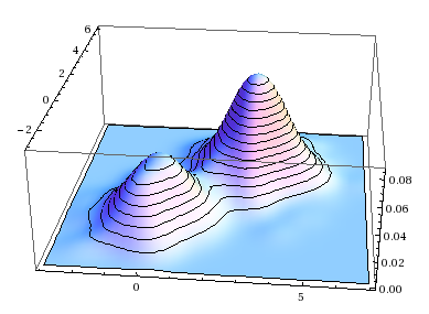
A single multivariate normal distribution has a single “hill” or “bump” located at $\boldsymbol{\mu}_i$; in contrast, a GMM is a multimodal distribution with on distinct bump per class. (Sometimes you get fewer than $k$ distinct local maxima in the p.d.f., if the bumps are sufficiently close together or if the weight of one class is zero or nearly so, but in general you get $k$ distinct bumps.) This makes it well suited to modeling data like that seen in our motivating example above, where there seems to be more than one region on high density.
We can view this is as a two-step generative process. To generate the $i$-th example:
- Sample a random class index $C_i$ from the categorical distribution parameterized by $\boldsymbol{\phi} = (\phi_1, … \phi_k)$.
- Sample a random vector $\mathbf{X}_i$ from the multivariate distribution associated to the $C_i$-th class.
The $n$ independent samples $\mathbf{X}_i$ are the row vectors of the matrix $\mathbf{X}$.
Symbolically, we write:
To fit a GMM model to a particular dataset, we attempt to find the maximum likelihood estimate of the parameters $\Theta$:
Because the $n \times m$ example matrix $\mathbf{X}$ is assumed to be a realization of $n$ i.i.d. samples from $f_{GMM}(\mathbf{x})$, we can write down our likelihood function as
We know that $\mathbf{X}_i$ has a multivariate normal distribution with parameters determined by the class, so the conditional probability $P(\mathbf{X}_i|C_i=j)$ can be written down pretty much directly from the definition:
Obtaining a formula for $P(C_i=j|\mathbf{X}_i)$ requires a little more work. We know that the unconditional probability is given by the parameter vector $\boldsymbol{\phi}$:
So using Bayes’ theorem, we can write this in terms of equation (7):
If we substituted equation (7) into (9) we could get a more explicit but very ugly formula, so I leave that to the reader’s imagination.
Equations (6), (7), and (9), when taken together, constitute the complete likelihood function $\mathcal{L}(\Theta;\mathbf{X})$. However, these equations have a problem - they depend on the unknown random variable $C_i$. This variable tells us which class each $\mathbf{X}_i$ was drawn from and makes it much easier to reason about the distribution, but we don’t actually know what $C_i$ is for any $i$. This is called a latent random variable and its presence in our model causes a kind of chicken-and-egg problem. If we knew $\boldsymbol{\mu}_j$ and $\Sigma_j$ for $j = (1, 2, …, k)$ then we could make a guess about what $C_i$ is by looking at which $\boldsymbol{\mu}_j$ is closest to $\mathbf{X}_i$. If we knew $C_i$, we could estimate $\boldsymbol{\mu}_j$ and $\Sigma_j$ by simply taking the mean and covariance over all $X_i$ where $C_i = j$. But how can we estimate these two sets of parameters together, if we don’t know either when we start?
The EM Algorithm
The solution to our chicken-and-egg dilemma is an iterative algorithm called the expectation-maximization algorithm, or EM algorithm for short. The EM algorithm is actually a meta-algorithm: a very general strategy that can be used to fit many different types of latent variable models, most famously factor analysis but also the Fellegi-Sunter record linkage algorithm, item response theory, and of course Gaussian mixture models.
The EM algorithm requires us to introduce a pseudo-parameter to model the unknown latent variables $C_i$. Because $C_i$ can take on $k$ discrete values, this new parameter will be a $n \times k$ matrix where each element $w_{ij}$ is an estimate of $P(C_i = j|\mathbf{X}_i;\theta)$. Each element of this matrix represents the probability that the $i$-th data point came from cluster $j$. This pseudo-parameter is only used when fitting the model and will be discarded afterwards; in that sense it is not a true parameter of the model.
The EM algorithm then proceeds iteratively, with each iteration being divided into two steps: the E-step and the M-step. I will describe these in broad strokes first, so you can get a feel for the overall intent of the algorithm, then we will study each in more detail in the following sections.
In the E-step, we use our current best knowledge of the centers and shapes of each cluster to update our estimates of which data point came from which class. Concretely, we hold $\boldsymbol{\mu}_j$ and $\Sigma_j$ fixed and update $w_{ij}$ and $\boldsymbol{\phi}$.
In the M-step, we use our current best knowledge of which class each point belongs to to update and improve our estimates for the center and shape of each cluster. Concretely, we use $w_{ij}$ as sample weights when updating $\boldsymbol{\mu}_j$ and $\Sigma_j$ by taking weighted averages over $X$. For example, if $w_11 = 0.01$ and $w_11 = 0.99$ we know that the data point $X_1$ is unlikely to be in class 1, but very likely to be in class 2. Therefore, when estimating the center of the first class $\boldsymbol{\mu}_1$ we give $X_1$ almost negligible weight, but when estimating the center of the second class $\boldsymbol{\mu}_2$ we give $X_1$ almost full weight. This “pulls” the center of each cluster towards those data points which are considered likely to be part of that cluster.
Visually, the iterative process looks something like this:

With each iteration, the algorithm improves its estimate of where the clusters are, which in turn allows it to make better guesses about which points are from which clusters, which in turn allows it to further refine its estimate of the center and shape of each cluster, and so on ad infinitum.
This process is guaranteed to converge a (local) maximum likelihood because of the ratchet principle: at each step, likelihood can only increase and never decrease. This can be viewed as a type of coordinate ascent. These maxima are not unique, and GMM will tend to converge to different final solutions depending on initial conditions.
One resource on GMM and the EM algorithm I used was this Stanford lecture by Andrew Ng. I’ve linked to the part of the lecture where he shows this update step because that is most relevant to implementing the algorithm but the whole lecture is worth watching if you want to understand the concepts. Another good resource on the fundamentals of the EM algorithm is this slide deck; it provides a simple example that can be worked by hand which I found to be a great way to build intuition before tackling the much more complicated problem of applying the EM algorithm to GMM.
We will now treat the E-step and M-step for the particular case of the GMM in detail.
E-step
Given the that centroid $\boldsymbol{\mu}_j$ and covariance matrix $\Sigma_j$ for class $j$ is fixed, we can update $w_{ij}$ by simply calculating the probability that $X_i$ came from each class and normalizing:
The conditional probablity $P(\mathbf{X}_i|K=j)$ is simply the multivariate normal distribution $\mathbf{X}_i ~ \mathcal{N}(\mu_i, \Sigma_i)$ so we can use equation (4) above to calculate the probability density for each class, and then divide through by the total to normalize each row of $\mathbf{X}$ to 1. This gives us a concrete formula for the update to $w_ij$:
The probability of each class $\phi$ can then be estimated by averaging over all examples in the training set:
M-step
Forget about the past estimates we had for $\boldsymbol{\mu}_j$ or $\Sigma$. Unlike gradient descent, the EM algorithm does not proceed by making small changes to the previous iteration’s parameter estimates - instead, it makes a bold leap all the way to the exact estimate - but only in certain dimensions. In the M-step, we will calculate the ML estimates for $\boldsymbol{\mu}_j$ or $\Sigma$ assuming that $w_{ij}$ is held constant.
How can we make such a leap? Well, we have a matrix of $n$ observations $\mathbf{X}_i$ with weights $w_i$ which we believe came from a multivariate distribution $\mathcal{N}(\vec{\mu}, \mathbb{\Sigma})$. That means we can use the familiar formulas:
These are in fact the ML estimate for these parameters for the multivariate normal distribution. As such, we don’t need to worry about learning rate or gradients as we would with gradient descent because these estimates are already maximal! This is one of the neatest things about this algorithm.
Implementation
Turning the above mathematics into a working implementation is straight
forward. The below program corresponds almost one-to-one (one line of code for
one equation) with the above mathematics. The equations (11), (12) are used in
the e_step() method and equations (13) and (14) are used in the m_step()
method.
One detail I did not treat above is initialization - while $\boldsymbol{\phi}$ and $w_{ij}$ can use simple uniform initialization, for $\boldsymbol{\mu}$ it is better to choose a random index $i_j$ uniformly from $1$ to $n$ for each class and then initialize $\boldsymbol{\mu}_j = X_{i_j}$. This ensures that each cluster centroid is inside the support of the underlying distribution and that they are initially spread out randomly throughout the space.
import numpy as np
from scipy.stats import multivariate_normal

class GMM:
    def __init__(self, k, max_iter=5):
        self.k = k
        self.max_iter = int(max_iter)

    def initialize(self, X):
        self.shape = X.shape
        self.n, self.m = self.shape

        self.phi = np.full(shape=self.k, fill_value=1/self.k)
        self.weights = np.full( shape=self.shape, fill_value=1/self.k)

        random_row = np.random.randint(low=0, high=self.n, size=self.k)
        self.mu = [  X[row_index,:] for row_index in random_row ]
        self.sigma = [ np.cov(X.T) for _ in range(self.k) ]

    def e_step(self, X):
        # E-Step: update weights and phi holding mu and sigma constant
        self.weights = self.predict_proba(X)
        self.phi = self.weights.mean(axis=0)

    def m_step(self, X):
        # M-Step: update mu and sigma holding phi and weights constant
        for i in range(self.k):
            weight = self.weights[:, [i]]
            total_weight = weight.sum()
            self.mu[i] = (X * weight).sum(axis=0) / total_weight
            self.sigma[i] = np.cov(X.T,
                aweights=(weight/total_weight).flatten(),
                bias=True)

    def fit(self, X):
        self.initialize(X)

        for iteration in range(self.max_iter):
            self.e_step(X)
            self.m_step(X)

    def predict_proba(self, X):
        likelihood = np.zeros( (self.n, self.k) )
        for i in range(self.k):
            distribution = multivariate_normal(
                mean=self.mu[i],
                cov=self.sigma[i])
            likelihood[:,i] = distribution.pdf(X)

        numerator = likelihood * self.phi
        denominator = numerator.sum(axis=1)[:, np.newaxis]
        weights = numerator / denominator
        return weights

    def predict(self, X):
        weights = self.predict_proba(X)
        return np.argmax(weights, axis=1)
Model Evaluation
We’ll use the famous iris dataset as a test case. This is the same dataset used as a motivating example at the beginning of the article, although I did not name it at that time. The iris dataset has labels, but we won’t expose them to the GMM model. However, we will use these labels in the next section to discuss the question, “were we able to discover the class labels through unsupervised learning?”
from scipy.stats import mode
from sklearn.metrics import confusion_matrix
import matplotlib.pyplot as plt
from sklearn.datasets import load_iris
iris = load_iris()
X = iris.data
Fit a model:
np.random.seed(42)
gmm = GMM(k=3, max_iter=10)
gmm.fit(X)
Plot the clusters. Each color is a cluster found by GMM:
def jitter(x):
    return x + np.random.uniform(low=-0.05, high=0.05, size=x.shape)

def plot_axis_pairs(X, axis_pairs, clusters, classes):
    n_rows = len(axis_pairs) // 2
    n_cols = 2
    plt.figure(figsize=(16, 10))
    for index, (x_axis, y_axis) in enumerate(axis_pairs):
        plt.subplot(n_rows, n_cols, index+1)
        plt.title('GMM Clusters')
        plt.xlabel(iris.feature_names[x_axis])
        plt.ylabel(iris.feature_names[y_axis])
        plt.scatter(
            jitter(X[:, x_axis]),
            jitter(X[:, y_axis]),
            #c=clusters,
            cmap=plt.cm.get_cmap('brg'),
            marker='x')
    plt.tight_layout()

plot_axis_pairs(
    X=X,
    axis_pairs=[
        (0,1), (2,3),
        (0,2), (1,3) ],
    clusters=permuted_prediction,
    classes=iris.target)
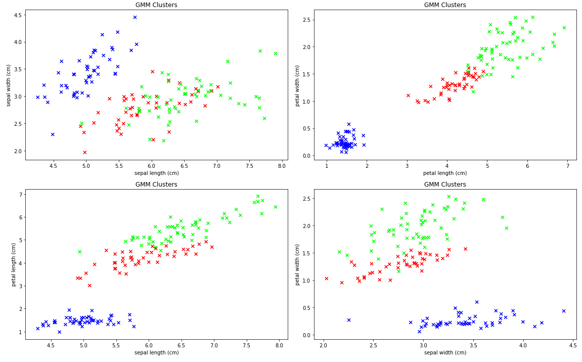
Well, the model certainly found something.
One thing we can say for sure is that the GMM model does find clusters of related points. It does a particularly good job placing the visually separate points in their own (blue) cluster, but the story with the other two clusters in the upper right is less clear-cut.
Comparing to True Class Labels
Are the clusters discovered by the GMM model meaningful? Are they correct? For a real-world unsupervised learning problem, these questions can be hard to answer.
However, it so happens that the iris dataset we used is actually labeled. True, we didn’t make use of these labels when training the GMM model. Furthermore, those classes are associated with different distributions in the 4 observed variables in a way that closely matches the assumptions of the GMM. So even if we can’t ask about “meaning” and “correctness”, we can at least ask a closely related question: “did this unsupervised learning algorithm (re-)discover the known structure of this (iris) data set?”
First, a bit of book-keeping. The cluster indexes found by the model are in random order. For convenience when comparing them to true class labels, we will permute them to be as similar as possible to true class labels. All this is doing is swapping, say, 0 for 2 so that 0 means the same thing for both the clusters and for the original class labels. It’s not important, but it does make comparisons a little bit easier.
permutation = np.array([
    mode(iris.target[gmm.predict(X) == i]).mode.item()
    for i in range(gmm.k)])
permuted_prediction = permutation[gmm.predict(X)]
print(np.mean(iris.target == permuted_prediction))
confusion_matrix(iris.target, permuted_prediction)

0.96
array([[50,  0,  0],
       [ 0, 44,  6],
       [ 0,  0, 50]])
For the random seed 42 (used above when the trained the GMM model) this results in the very promising 96% agreement! However, if we 1,000 random trials, varying the seed each time, we can see that cluster-to-labels agreement actually varies at random from 0.52 to 0.99 with a mean of 0.74.
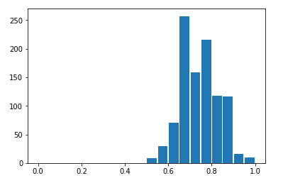
This is a little disappointing. We started from a dataset which really was the aggregation of three different classes, and while our unsupervised learning algorithm was discover three clusters, the agreement between reality and our model is only around 3⁄4. That means we can’t reliably reconstruct the true structure of this dataset using this technique. In contrast, a supervised learning algorithm could have easily found a class boundary with an accuracy of 99%. That suggests that if we run an unsupervised learning algorithm on a real-world data set and it finds some clusters for us, we should be suspicious that they represent “true” classes in the real world. In fact, unsupervised learning algorithms are subject to a large number of caveats and limitations which I’ll digress briefly to enumerate.
Limitations
All unsupervised learning methods known today share certain limitations.
First, they tend to rely on the researcher choosing certain arbitrary complexity parameters such as the number of clusters $k$. Worse still, while there are techniques for picking these complexity parameters, they are heuristic and often unsatisfying in practice. It can be very hard to tell if an unsupervised learning method is “overfitting”, because “overfit” doesn’t even have a precise definition for unsupervised learning problems.
Second, there are no hard metrics like accuracy or AUC that let you compare models across different families. While each unsupervised learning algorithm will have its own internal metrics which they try to optimize such as variance explained or perplexity, these usually can’t be meaningful compare two models that use two different algorithms or with different complexity parameters. This makes model selection a fundamentally subjective task - to decide that, say, t-SNE is doing a better job than $k$-means on a given data set, the modeler is often reduced to eyeballing the output.
Third and finally, the factors and/or clusters discovered by unsupervised learning algorithms are often unsatisfying or counter-intuitive and don’t necessarily line up with human intuition. Another way of saying the same thing is that if a human goes through and creates labels $\mathbf{Y}$ for the training set $\mathbf{X}$ after the unsupervised learning algorithm has been applied to it, they are not very likely to come up with the same factors or clusters. In general, humans tend to come up with rules that “make sense” but don’t explain as much variance as possible, while algorithms tend to find “deep” features that do explain a lot of variance but have complicated definitions that are hard to make sense of.
These seem like serious criticisms; does this mean we shouldn’t use unsupervised learning? Well, I won’t tell you that you categorically should never use it, but you should know what you’re getting into. By default, it tends to produce low-quality, hard-to-interpret models that cannot really be defended due to number of subjective decisions needed to make them work at all.
On the other hand, unsupervised learning can be extremely helpful during exploratory research; also, in the form of representation learning, it can sometimes accelerate learning or improve performance, or allow models to generalize from an extremely limited labeled training set. For example, a sentiment analysis model trained on only a few hundred reviews may only see the word “sterling” once, but if it uses a word embedding model like Word2Vec, it will understand that “stupendous” is broadly a synonym for “good” or “great”, and will therefore be able to correctly classify a future example with the word “stupendous” - which did not appear even once in the training set - as likely having positive sentiment. While success stories like this are possible, in general unsupervised learning requires more expertise, more manual tuning, and more input from domain experts in order to create value, when compared to supervised learning projects.
Unfortunately, we do not always have the labels necessary for supervised learning, and the datasets available may be too large, too high dimensional, or too sparse to be amenable to traditional techniques; it is in these situations where the benefits of unsupervised learning can outweigh the negatives.
Conclusion
In this article, we have seen how unsupervised learning differs from supervised learning and the challenges that come along with that. We discussed a method for posing an unsupervised learning problem as an maximum likelihood optimization, and described and implemented the EM algorithm often used to solve these otherwise intractable problems. We made the EM algorithm concrete by implementing one particular latent variable model, the Gaussian mixture model, a powerful unsupervised clustering algorithm. We’ve seen first hand that the clusters identified by GMMs don’t always line up with what we believe the true structure to be; this lead to a broader discussion of the limitations of unsupervised learning algorithms and the difficulty getting value out of them.
In the next article in this series, we’ll continue our discussion of unsupervised learning algorithms by implementing the other kind of unsupervised learning algorithm besides clustering: a dimensionality reduction algorithm.