
Kaprekar's Magic 6174
Kaprekar’s routine is a simple arithmetic procedure on four digit numbers which rapidly converges to the fixed point 6174, known as the Kaprekar constant. Unlike other famous iterative procedures such as the Collatz function, the ad hoc nature of the Kaprekar routine doesn’t hint at fundamental mathematical discoveries yet to be made.
Rather, its charm lies in its intuitive definition (requiring no more than elementary mathematics,) its oddly off-center fixed point of 6174, and its surprisingly rapid convergence (which requires only five iterations on average and never more than seven.)
The routine itself is simple. Given a four digit number, say 8352, we first place the digits in descending order to obtain a larger 4-digit number (8532) and then in ascending order to obtain a smaller 4-digit number (2358) and then subtract the smaller from the larger to obtain the result. (8532-2358 = 6174). This represents one iteration in the routine. The process is repeated until the output is the same as the input, at which point we can stop, because we have reached the fixed point and the same result will recur endlessly.
There are two edge cases to consider. In order for the procedure to work correctly, we need to treat numbers less than 100 (and which therefore have three or fewer digits when written normally) as if they indeed had four digits and were padded with leading zeros. For example, we would treat the number 42 as having the four digits “0042” and take 4200 - 0024 to obtain 4176. Also, if the Kaprekar procedure is applied to numbers with all the same digits, such as 5555, then the result would be zero, which is inconvenient. For that reason, we exclude such numbers from the domain, and simply say that the function is undefined on them.
All of this can be succinctly and exactly expressed in a few lines of code:
def sort_digits(n: int, length: int) -> str:
    return ''.join(sorted(str(n).zfill(length)))


def k(n: int, length: int = 4) -> int:
    ascending = sort_digits(n, length)
    descending = ascending[::-1]
    return int(descending) - int(ascending)


def kaprekar(n, length: int = 4) -> tuple[int, int]:
    i = 0
    while True:
        m = k(n, length)
        if m == n:
            return i, m
        i = i+1
        n = m
Note that k(n) computes one iteration of the routine and returns the next
number in the series, while kaprekar(n) returns both the number of iterations
it takes to reach the fixed point and the value of the fixed point itself as a
pair; for example, (5, 6174) means “reached the fixed point 6174 after 5
iterations.”
Implementing Kaprekar is easy. Showing that every valid four digit number reaches the fixed point 6174 is computationally trivial given there are only 9,990 such numbers. Explaining why it should have a unique fixed point and why the convergence is so rapid is not so simple. For example, it would be entirely plausible for it to converge to a cycle, oscillating forever between two or more values for ever, or for it to converge to one of several distinct fixed points or cycles depending on the starting number.
It’s also not clear why the convergence should be so rapid: if each iteration cut down the number of surviving numbers by half, it would still take about 13 iterations to collapse to a single value. In that sense, Kaprekar converges “surprisingly” quickly.
Let’s see if we can say anything interesting about the nature of the convergence. We’ll use data visualization to develop intuition and formulate hypotheses, then write simple programs to validate them.
Number of Iterations
We’ll start with a simple histogram:
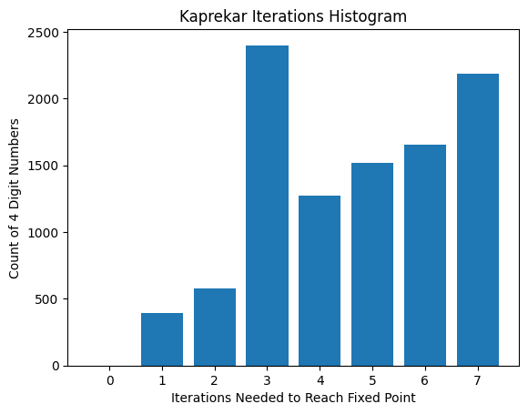
Most numbers are “far” from the fixed-point and require many iterations to reach it.
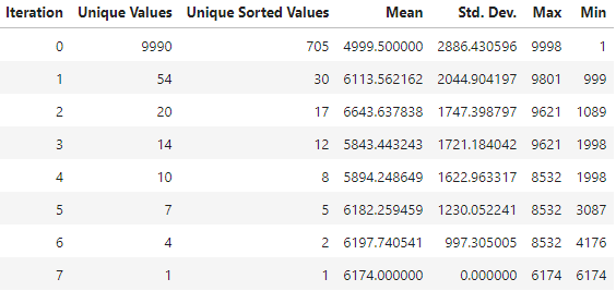
Next, let’s try to get a sense of how rapid convergence is. We start with the full pool of 9,990 distinct valid numbers, and for each iteration we plot (using a log scale) how many unique numbers remain after $k$ iterations:
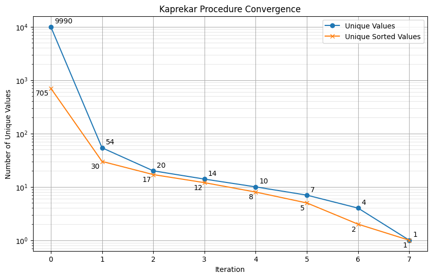
This graph also shows the number of unique “sorted” values, where “sorted” means that the digits of the number where sorted. It is possible to think of the Kaprekar routine as two separate steps: it first sorts the digits of the number, then it differences it with its reverse. That means that it essentially ignores the original order of digits; any two numbers with the same set of digits, regardless of order, will necessarily have the same result. Numbers like 4277, 2477, 7427, and 7274 will all map the same number. The digit sorting step is responsible for the lions share of collisions; in fact, we can see that in the very first iteration it has already reduced the set of valid numbers from 9,990 to 705 - reducing the pool by 97%.
However, the second step, differencing with the reverse, is also responsible for a large number of collapses. After the first differencing step, we’ve gone from 705 unique sorted values to only 54, reducing the total pool of survivors by another 92%. Taken together, these eliminate 99.5% of all unique values in the first iteration alone.
After that, convergence slows considerably. The slope on the log scale plot is about 1⁄2, which means that each subsequent iteration cuts the pool of unique numbers roughly in half.
The above visualizations are good high level summaries but we want to investigate the structure in more detail, ideally all the way down to the individual numbers. To visualize all numbers up to 9999 on a single graph, we take the first two digits as the x coordinate and the last two digits as the y coordinate and plot them on a 100x100 grid. (I didn’t invent this - it seems to be quite a common way to visualize the Kaprekar routine, although I’m not sure where it originated.)
# reshape counts into a 2D grid
data = np.array([0] + kaprekar_iteration_counts(4))
reshaped_data = data.reshape((100, 100))

# plot the grid
plt.figure(figsize=(10, 8))
plt.imshow(reshaped_data, cmap='coolwarm', vmin=0, vmax=7, aspect='equal')
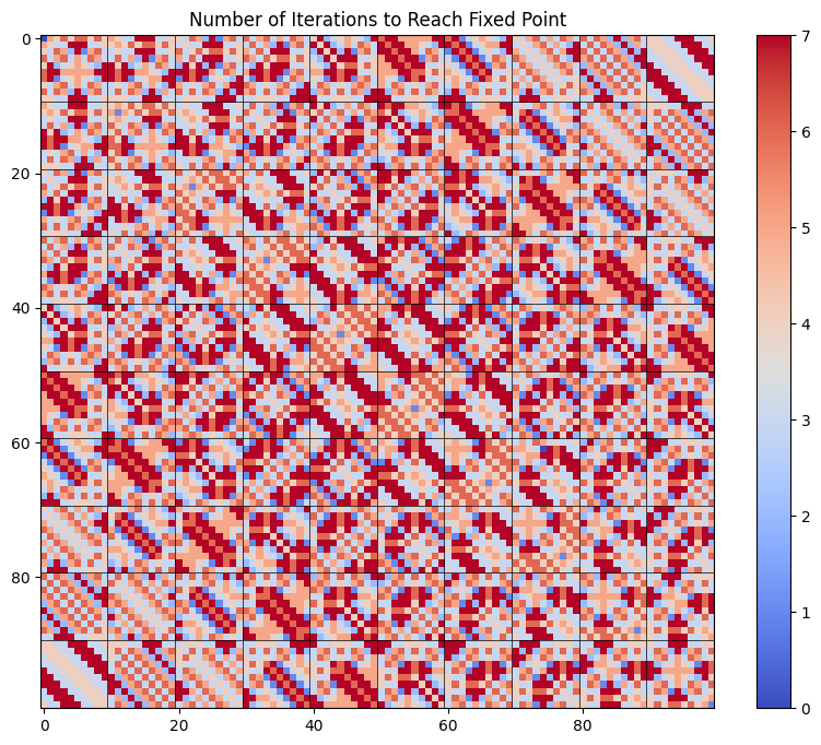
An interesting structure emerges: there are many diagonal streaks that share the exact same color. Is there something about two points being diagonal neighbors in this 100x100 space that makes them more likely to collapse?
Structure of Convergence
Another way to use the 100x100 grid is to assign a color to every unique number after $k$ iterations. If two pixels have the same color, we know they will collide in $k$ iterations or fewer.
First iteration:
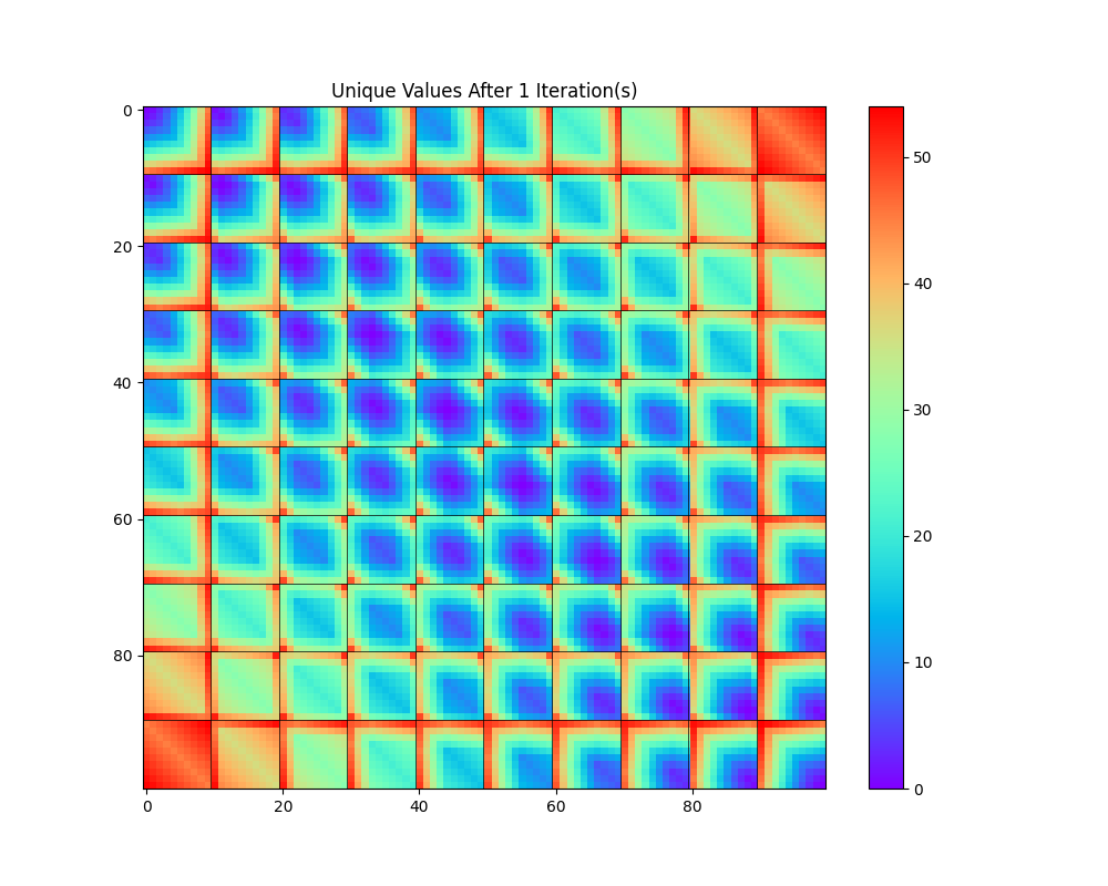
See if you can mentally visualize this in four dimensions by first stacking all the cells in a row to get a 3D shape, then again for each columns to get a 4D shape. You should see a kind of 4-dimensional blue football with red around the corners. Numbers where all four digits are similar (like 4445) map to low numbers (like 0999), while numbers with dissimilar digits (like 0009) map to high numbers (like 8991.)
To avoid duplicating this visual seven times, I’ve compressed it into an animation:

This allows us to see collapses occurring with each iteration and observe the complex but obviously non-random structure that emerges. (The static images for each iteration are available in the Jupyter notebook.)
The diagonal structure we notice above seems prominent in this visualization as well; in fact, it seems to get even more pronounced as the number of iterations increases. What is going on there?
While the 100x100 is good for getting a gestalt impression of the whole, it’s hard to read off individual transitions or trace the orbits of individual numbers through the iteration. For a more detailed deep dive, we can use Graphviz to visualize the exact structure of collapses. To avoid overwhelming the visualization, let’s only show the 54 unique numbers that survive the first iteration:
# Initialize the unique colors set and the arrows set
unique_colors = set()
arrows = set()

# Generate the 'ukx' array with unique Kaprekar values
ukx = np.unique([k(x, 4) for x in range(1, 10000) if not identical_digits(x, 4)])

for x in ukx:
    color_number = sort_digits(x, 4)
    color = color_map[color_number]
    arrows.add(f'{x} [fillcolor="{color}", style=filled]')
    arrows.add(f'{x} -> {k(x)}')

# Create and print the graph definition
print('digraph G {')
for arrow in arrows:
    print('   ', arrow)
print('}')
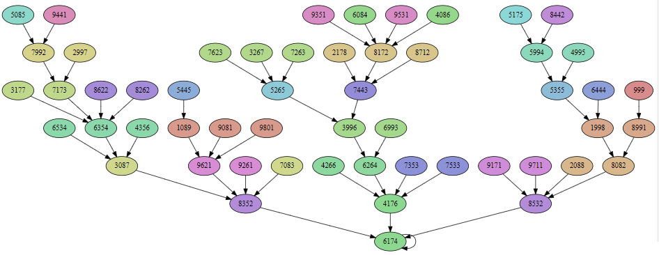
On this graph, each number is a node, and you can follow the arrow to see where the Kaprekar function sends that number. The nodes are color-coded according to their sorted digits, so any two numbers which are the same modulo the digit sorting operation will be the same color. That makes it obvious that digit sorting is still responsible for a large number of collapses. For example, we can see that 7623, 3267, and 7263 (shown in light green) all map to 5265, and that is entirely due to them have the same set of digits, just in a different order.
It’s the collapses which are not due to digit sorting which are really fascinating, though. Why do 7173 and 8262 collapse together, for example? If you look closely, these numbers do have a relationship; each digit is different by exactly 1:
| 7173 | 8262 | Difference |
|---|---|---|
| 7 | 8 | +1 |
| 1 | 2 | +1 |
| 7 | 6 | -1 |
| 3 | 2 | -1 |
This same pattern occurs in many other places on the graph as well. That can’t be a coincidence, can it?
Recall the diagonal patters that characterized the above 100x100 visualization. What does it mean for two points to be “diagonal neighbors” on that visualization? Doesn’t that also mean some of their digits also differ by only 1?
Diagonal Structure
The diagonal streaks in the above suggest something about the structure.
Let’s say you add one to both the largest and smallest digit. After you apply the Kaprekar procedure, that “+1” will cancel out, because the largest and smallest digits will be aligned by the process of flipping the digits around. Thus, we should expect the result of k() to be the same.
def are_diagonal(x, y, length=4) -> bool:
    if length != 4:
        raise NotImplementedError("only implemented for length=4 so far.")

    # Sort the digits of each number
    sorted_x = sort_digits(x, length=length)
    sorted_y = sort_digits(y, length=length)

    # Compute the differences between the sorted digits
    differences = [int(b) - int(a) for a, b in zip(sorted_x, sorted_y)]
    for d in differences:
        if abs(d) != 1:
            return False

    return all([ d1 == d2 for (d1, d2) in zip(differences, differences[::-1]) ])
We can implement a proof by exhaustion to empirically verify this insight:
count_misses = 0
count_hits = 0
neighbors = []

for z in sorted_valid_numbers:
    kz = k(z)
    for w in sorted_valid_numbers:
        if w < z and are_diagonal(z, w):
            kw = k(w)

            neighbors.append({ 'z': z, 'w': w, 'k(z)': kz, 'k(w)': kw })
            if kz != kw:
                print(f'z={z} w={w} k(z)={kz} k(w)={kw}')
                count_misses += 1
            else:
                count_hits += 1

print(f'hits: {count_hits}, misses: {count_misses}')
neighbors_df = pd.DataFrame(neighbors)
This verifies this theorem for us - if two numbers are diagonal neighbors, then the Kaprekar is guaranteed to send them to the same value, causing a collision.
Collisions
There are two main mechanisms for collisions:
- Digit Sorting
- Diagonal Neighbors
There are also many “random” collisions on the first iteration. However, after the first iteration, every collision is explained by one of those two mechanisms, as you can verify yourself from the graph above.
I think this explains the extraordinary rapid convergence on the sequence - there are two distinct and common ways to have a collision between any two numbers, so a Birthday problem style argument all but guarantees that there will be collisions in any larger set of numbers.
This kind of pseudo-probabilistic argument doesn’t offer any guarantees of course. There is a still an element of chance, especially in the last few iterations. We know this because if we look at variants of the problem (different number of digits than 4, bases other than base-10) then we often find there is not a unique fixed point. But it does make it much less surprising that it should rapidly converge.
Is there any deep reason why there is a unique fixed point for 4-digit base-10 numbers? The fact that other variants ($n$-digits base-$m$ numbers) often have cycles suggest not. In fact, it’s more like a weak anthropic principle - the only reason this particular combination caught Kaprekar’s attention is because it does happen to have a unique fixed point, while (for example) 3 or 5 digit numbers are ignored.
Why is the fixed point 6174? I originally thought there was some significance to the fact that this was quite close to the average $k(n)$ - that is to say, if you choose a random number $n$ uniformly between 1 and 9999, and calculate $k(n)$, then the expected value is 6108 - quite close to the fixed point. This is fairly intuitive when you consider that sorting the digits of a number in descending order tends to increase it (to about 8054 on average) and sorting them ascending tends to decrease it (to an average of 1946) And the Kaprekar routine takes the average of these two (which is where 6108 comes from.)
However, there’s no real evidence of the Kaprekar routine converging to this mean or really even narrowing significantly across iterations, except by the inevitable winnowing as the number of unique values decreases as collisions occur. (If you select a finite sample from a uniform distribution and calculate the range, it will on average be smaller than the width of the original distribution; range is an optimal but biased estimator of the width of a uniformly distributed random variable.) It jumps up and down all over the place and the fact that it happens to end up quite close to the mean feels more like luck than any kind of convergence - insofar “luck” has any meaning for a deterministic process.
Conclusion
The observation that “diagonal neighbors” is the primary mechanism for collapses (other than digit sorting, obviously) is interesting, and it arose directly from doing the 100x100 grids and interpreting the patterns found there. The animation showing unique values collapsing it attractive and eye-catching but hard to interpret. The color-coded graph showing individual transitions is complex but rewards close study and the “diagonal neighbor” structure is even more apparent on this graph than on the 100x100 views.
Source code for this project is available as a Jupyter notebook (.html, .ipynb).