
ML From Scratch, Part 2: Logistic Regression
In this second installment of the machine learning from scratch we switch the point of view from regression to classification: instead of estimating a number, we will be trying to guess which of 2 possible classes a given input belongs to. A modern example is looking at a photo and deciding if its a cat or a dog.
In practice, its extremely common to need to decide between \(k\) classes where \(k > 2\) but in this article we’ll limit ourselves to just two classes - the so-called binary classification problem - because generalizations to many classes are usually both tedious and straight-forward. In fact, even if the algorithm doesn’t naturally generalize beyond binary classification (looking at you, SVM) there’s a general strategy for turning any binary classification algorithm into a multiclass classification algorithm called one-vs-all. Let’s agree to set aside the complexities of the multiclass problem and focus on binary classification for now.
The binary classification problem is extremely central in machine learning and in this series we’ll be looking at no fewer than four different “serious” classification algorithms. In an undergraduate machine learning class, you’d probably work through a few “non-serious” or “toy” algorithms that have only have historical or pedagogical value: the one-unit perceptron, linear discriminant analysis, the winnow algorithm. We will omit those and jump straight to the simplest classification that is in widespread use: logistic regression.
I say, “simplest,” but most people don’t think of LR as “simple.” That’s because they’re thinking of it use within the context of statistical analysis and the design and analysis of experiments. In those contexts, there’s a ton of associated mathematical machinery that goes along with validating and interpretting logistic regression models, and that stuff is complicated. A good book on that side of logistic regression is Applied Logistic Regression by Hosmer et al.. But if you simply want to fit data and make predictions then logistic regression is indeed a very simple model: as we’ll see, the heart of the algorithm is only a few lines of code.
Despite it’s simplicity, it’s important for three reasons. First, it can be surprisingly effective. It’s not uncommon for some state-of-the-art algorithm to significantly contribute to global warming by running a hyperparameter grid search over a cluster of GPU instances in the cloud, only to end up with a final model with only slightly lower generalization error than logistic regression. Obvious, this isn’t always true, otherwise there would be no need to study more advanced models. For example, LR tends to get only ~90% accuracy on the MNIST handwritten digit classification problem, which is much lower than either humans or deep learning. But in the many cases for which it is true, it’s worth asking if the problem is amenable to more advanced machine learning techniques at all.
The second reason logistic regression is important is that it provides a important conceptual foundation for neural networks and deep learning, which we’ll visit later in this series.
The third and final reason is that it cannot be solved with linear algebra so serves as a legitimate reason to introduce one of the most important tools in machine learning: gradient descent. Just as in part 1, we’ll take the hard path through the mud and develop (step-by-step) an algorithm which could actually be used in production without too much embarrassment.
The Logistic Function
Before we get to the regression model, let’s take a minute to make sure we have a good understanding of the logistic function and some of its key properties.
The logistic function (also called the sigmoid function) is given by:
\[ \sigma(x) = \frac{1}{1 + e^{-x}} \]
It looks like this:
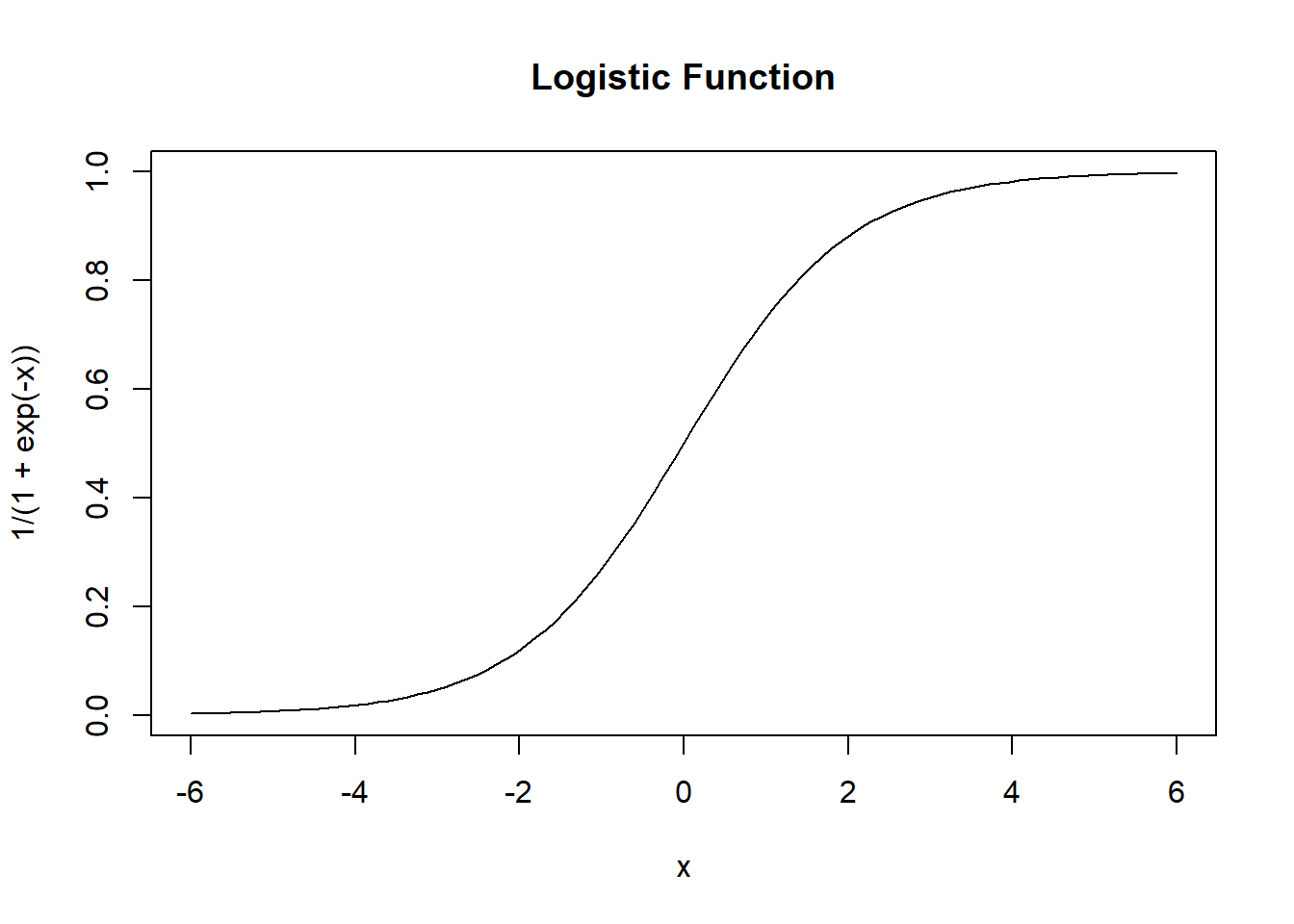
First, we note that its domain is \((-\infty, +\infty)\) and its range is \((0, 1)\). Therefore its output will always be a valid probability. Note also that \(\sigma(0) = 0.5\) so if we interpret the output as a probability, all negative numbers map to probabilities that are unlikely, while all positive numbers map to probabilities that are likely, while zero maps to exactly even odds.
A few lines of simple algebra will show that its inverse function (also called the “logit” function) is given by
\[ \sigma^{-1}(x) = \ln{\frac{x}{1-x}} \]
Note that if \(x = e^p\) where \(p\) is a probability between 0 and 1, then we have
\[ \sigma^{-1}(e^p) = \frac{p}{1-p} \]
Where the right hand side is an odds ratio. So one interpretation of the logistic function is that it is the bijection between log odds ratios to probabilities.
For example, if something has a probability of 0.2, then it has 4:1 odds, therefore the odds ratio is 4, therefore the log odds ratio of \(\ln 4 = -1.39\). So \(\sigma(0.2) = -1.39\).
The logistic function also has a pretty interesting derivative. The slickest way to show the following result is to use implicit differentiation, but I’ll show a longer and less magical derivation which only uses the chain rule and basic algebra.
\[ \begin{split} \frac{d}{dx} \sigma(x) & = \frac{d}{dx} \frac{1}{1 + e^{-x}} \\ & = \frac{-e^{-x}}{( 1+ e^{-x})^2} \\ & = \frac{1}{1 + e^{-x}} \frac{1 + e^{-x} - 1}{ 1+ e^{-x}} \\ & = \frac{1}{1 + e^{-x}} \Big( \frac{1 + e^{-x}}{1+ e^{-x}} - \frac{1}{ 1+ e^{-x}} \Big) \\ & = \frac{1}{1 + e^{-x}} \Big( 1 - \frac{1}{ 1+ e^{-x}} \Big) \\ & = \sigma(x) ( 1 - \sigma(x) ) \end{split} \]
So we can see that \(\sigma'(x)\) can expressed as a simple quadratic function of \(\sigma(x)\). It’s not often that a derivative can be most conveniently expressed in terms of the original function, but it turned out to be the case here. This apparently useless fact is actually quite important numerically because it means we can calculate \(\sigma'(x)\) with only a single multiplication assuming that we already know \(\sigma(x)\).
For our Python implementation, we will need a vectorized implementation of
\(\sigma()\). This function applies the sigmoid function element-wise to every
element in a numpy.ndarray of any shape.
import numpy as np

def sigmoid(z):
    return 1 / (1 + np.exp(-z))
Statistical Motivation
Let \(Y\) be a discrete random variable with support on \(\{0, 1\}\) and let \(X\) be a random \(m\)-vector. Let’s assume that the joint probability distribution \(F_{X,Y}\) of \(X\) and \(Y\) has the following sigmoid form for some real-valued vector \(\Theta\):
\[ E[Y|X] = P(Y=1|X) = \sigma(X\Theta) \]
Now let’s say \(\mathbf{X}\) is an \(n \times m\) matrix and \(\mathbf{y}\) is an \(n\)-vector such that \((\mathbf{y}_i, \mathbf{X}_i)\) are \(n\) realizations sampled independently from \(F_{X,Y}\); then we can write down the likelihood function:
\[ L(\Theta; \mathbf{X}, \mathbf{y}) = \prod_{i=1}^n P(Y=1|X=\mathbf{X}_i)^{\mathbf{y}_i} P(Y=0|X=\mathbf{X}_i)^{(1 - \mathbf{y}_i)} \]
I should probably explain the notational trick used here: because \(y \in \{0, 1\}\), the first factor will be reduced to a constant \(1\) if \(y = 0\) and likewise the second term will be reduced to a constant \(1\) if \(y = 1\). So putting \(y\) and \(1-y\) in the exponent is merely a compact way of writing the two mutually exclusive scenarios without an explicit if/else.
We can simplify this expression by taking the log of both sides and working with the log-likelihood \(\ell\) from now on:
\[ \ell(\Theta; \mathbf{X},\mathbf{y}) = \ln L = \sum_{i=1}^n \mathbf{y}_i \ln P(Y=1|X=\mathbf{X}_i) + (1 - \mathbf{y}_i) \ln (1 - P(Y=1|X=\mathbf{X}_i) \]
Substituting \(\hat{\mathbf{y}} = P(Y=1|X)\):
\[ \ell(\Theta; \mathbf{X},\mathbf{y}) = \ln L = \sum_{i=1}^n \mathbf{y}_i \ln \hat{\mathbf{y}}_i + (1 - \mathbf{\mathbf{y}}_i) \ln (1 - \hat{\mathbf{y}}_i) \]
Because \(\ln()\) is monotonically increasing, it suffices to minimize \(\ell(\Theta; \mathbf{X}, \mathbf{y})\) with respect to \(\Theta\) in order to find the maximum likelihood estimate. Because \(\ell\) is convex and has a continuous derivative, we can find this maximum by solving \(\nabla \ell = 0\).
\[ \begin{align} \frac{\partial \ell}{\partial \Theta} & = \sum_{i=1}^n \frac{\mathbf{y}_i}{\hat{\mathbf{y}}_i} \frac{\partial \hat{\mathbf{y}}_i}{\partial \Theta} - \frac{(1-\mathbf{y}_i)}{(1-\hat{\mathbf{y}}_i)} \frac{\partial \hat{\mathbf{y}}_i}{\partial \Theta} \end{align} \]
We can use our earlier lemma \(\sigma'(x) = \sigma(x)(1-\sigma(x))\) for the partial derivative of \(\hat{y}\). Note also that because \(\hat{y}_i = \sigma(\mathbf{X}_i^T \Theta)\), we will pick up an additional \(\mathbf{X}_i\) from the chain rule when differentiating by \(\Theta\).
\[ \begin{align} \frac{\partial \ell}{\partial \Theta} = \sum_{i=1}^n \frac{\mathbf{y}_i}{\hat{\mathbf{y}}_i} \hat{\mathbf{y}}_i (1-\hat{\mathbf{y}}_i) \mathbf{X}_i - \frac{(1-\mathbf{y}_i)}{(1-\hat{\mathbf{y}}_i)} \hat{\mathbf{y}}_i (1-\hat{\mathbf{y}}_i) \mathbf{X}_i \end{align} \]
We can use simple algebra to simplify this a great deal, and in the end we are left with:
\[ \begin{align} \frac{\partial \ell}{\partial \Theta} & = \sum_{i=1}^n \mathbf{X}_i ( \mathbf{y}_i (1 - \hat{\mathbf{y}}_i) - (1 - \mathbf{y}_i) \hat{\mathbf{y}}_i ) \\ & = \sum_{i=1}^n \mathbf{X}_i ( \mathbf{y}_i - \mathbf{y}_i \hat{\mathbf{y}}_i - \hat{\mathbf{y}}_i + \mathbf{y}_i \hat{\mathbf{y}}_i) \\ & = \sum_{i=1}^n \mathbf{X}_i ( \mathbf{y}_i - \hat{\mathbf{y}}_i ) \\ & = \mathbf{X}^T ( \mathbf{y} - \hat{\mathbf{y}} ) \tag{1} \\ \end{align} \]
Equation (1) is the clearest way to express the gradient, but because \(\hat{\mathbf{y}}\) is an implicit function of \(\mathbf{X}\) and \(\Theta\) is can appear a little magical. A fully explicit version is:
\[ \frac{\partial \ell}{\partial \Theta} = \mathbf{X}^T ( \mathbf{y} - \sigma(\mathbf{X} \Theta) ) \tag{2} \]
In plain english, this says: go through the rows of \(\mathbf{X}\) one by one. For each row, figure out if the prediction \(\hat{\mathbf{y}}\) was too high or too low by computing the difference \(\mathbf{y}_i - \hat{\mathbf{y}}_i\). If it’s too high, subtract the row \(X_i\) from the gradient, and if it’s too low, then add the row \(X_i\) to the gradient, in each case weighting by the magnitude in the difference.
In theory, we can now find the minimum \(\hat{\Theta}\) by simply solving equation (3):
\[ \mathbf{X}^T ( \mathbf{y} - \sigma(\mathbf{X} \hat{\Theta}) ) = 0 \tag{3} \]
Unfortunately, unlike the normal equation of ordinary least squares, equation (3) cannot be solved by the methods of linear algebra due to the presence of the non-linear \(\sigma\) function. However, it is amenable to numerical methods, which we will cover in great detail below.
You may remark that equation (3) is almost suspiciously neat, but it’s not really an accident. The reason why we chose the logistic function in the first place was precisely so this result would drop out at the end. Indeed, there are other choices with an equally good theoretical basis, yet we chose logit because it’s simple and fast to calculate.
One such alternative, preferred by some statisticians and scientific specializations, is the probit link function, which uses the CDF of the normal distribution instead of sigmoid. However, in practice these curves are extremely similar, and if you showed me an unlabeled plot with both of them I could not for the life of me tell you which is which:
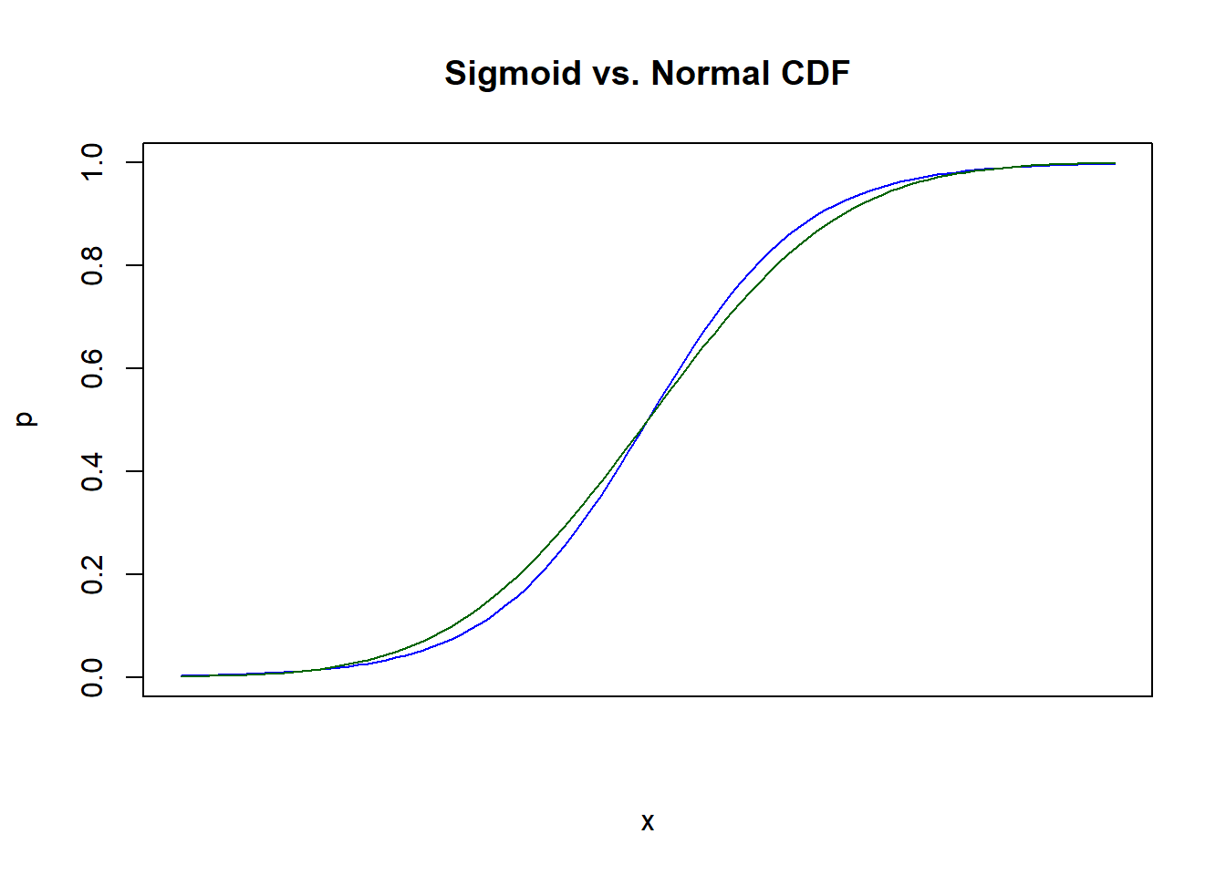
It’s worth bearing in mind that logistic regression is so popular, not because there’s some theorem which proves it’s the model to use, but because it is the simplest and easiest to work with out of a family of equally valid choices.
Gradient Descent
The state-of-the-art algorithm that we will use to solve (3) has a large number of moving parts and is somewhat overwhelming to understand at once. Therefore, we will implement it in layers, adding sophistication at each layers as well as taking benchmarks that will concretely demonstrate the value of each added complication. The layers will be:
- (Batch) Gradient Descent
- Minibatch Stochastic Gradient Descent
- Nesterov Accelerated Gradient
- Early Stopping
Batch Gradient Descent
Since we have both the loss function \(J\) we want to minimize and its gradient \(\nabla J\) we can use an algorithm called gradient descent to find a minimum.
Gradient descent is an iterative method that simply updates an approximation of \(\hat{\Theta}\) by taking a smalls step in the direction of steepest descent. Let us denote this sequence of approximations \(\hat{\Theta}_t\). Initialize \(\hat{\Theta}_0\) arbitrarily and use the following update rule for \(t>0\):
\[ \hat{\Theta}_{i+1} := \hat{\Theta}_i - \alpha \nabla \ell (\hat{\Theta}_i) \]
For some suitable learning rate \(\alpha\) this will always converge, and because \(\ell\) is convex it will in fact always converge to the unique global minimum \(\hat{\Theta}\) which is the maximum likelihood estimate for \(\Theta\).
class LogisticClassifier:
    def __init__(self, learning_rate=0.1, tolerance=1e-4, max_iter=1000):
        # gradient descent parameters
        self.learning_rate = float(learning_rate)
        self.tolerance = float(tolerance)
        self.max_iter = int(max_iter)

        # how to construct a the design matrix
        self.add_intercept = True
        self.center = True
        self.scale = True

        self.training_loss_history = []

    def _design_matrix(self, X):
        if self.center:
            X = X - self.means
        if self.scale:
            X = X / self.standard_error
        if self.add_intercept:
            X = np.hstack([ np.ones((X.shape[0], 1)), X])

        return X

    def fit_center_scale(self, X):
        self.means = X.mean(axis=0)
        self.standard_error = np.std(X, axis=0)

    def fit(self, X, y):
        self.fit_center_scale(X)

        # add intercept column to the design matrix
        n, k = X.shape
        X = self._design_matrix(X)

        # used for the convergence check
        previous_loss = -float('inf')
        self.converged = False

        # initialize parameters
        self.beta = np.zeros(k + (1 if self.add_intercept else 0))

        for i in range(self.max_iter):
            y_hat = sigmoid(X @ self.beta)
            self.loss = np.mean(-y * np.log(y_hat) - (1-y) * np.log(1-y_hat))

            # convergence check
            if abs(previous_loss - self.loss) < self.tolerance:
                self.converged = True
                break
            else:
                previous_loss = self.loss

            # gradient descent
            residuals = (y_hat - y).reshape( (n, 1) )
            gradient = (X * residuals).mean(axis=0)
            self.beta -= self.learning_rate * gradient

        self.iterations = i+1

    def predict_proba(self, X):
        # add intercept column to the design matrix
        X = self._design_matrix(X)
        return sigmoid(X @ self.beta)

    def predict(self, X):
        return (self.predict_proba(X) > 0.5).astype(int)
Grab some test-only dependencies:
# dependencies for testing and evaluating the model
from sklearn.datasets import load_breast_cancer
from sklearn.metrics import confusion_matrix, accuracy_score, roc_auc_score, roc_curve
import matplotlib.pyplot as plt

from sklearn.datasets import load_breast_cancer
from sklearn.metrics import confusion_matrix, accuracy_score, roc_auc_score, roc_curve
import matplotlib.pyplot as plt
%matplotlib inline
If we fit this naive model to a smallish dataset:
model = LogisticClassifier(tolerance=1e-5, max_iter=2000)
%time model.fit(X_train, y_train)
model.converged, model.iterations, model.loss
CPU times: user 2.78 s, sys: 3.31 s, total: 6.09 s Wall time: 3.07 s
(True, 1094, 0.063013434109990218)
So it took 1000 iterations and 3 seconds to converge. That’s not great, and we’ll see how to improve it in just a minute. First, though, let’s take a look at how the model performs on the test set:
p_hat = model.predict_proba(X_test)
y_hat = model.predict(X_test)
accuracy_score(y_test, y_hat)

0.9707602339181286
97% accuracy is quite good. We can get a slightly deeper look at this result by looking at the confusion matrix for the \(p<0.5\) decision rule:
| Actual Positive | Actual Negative | |
|---|---|---|
| Predicted Positive | 109 | 3 |
| Predicted Negative | 2 | 57 |
This tells us we’re doing roughly equally well at classifying negatives and positives so our high accuracy is not due simply to unbalanced class prevalence - the model has real insight. Nevertheless, we can try out different breakpoints to see if that makes any difference.
fpr, tpr, threshold = roc_curve(y_test, p_hat)
fpr = np.concatenate([[0], fpr])
tpr = np.concatenate([[0], tpr])
threshold = np.concatenate([[0], threshold])
plt.figure(figsize=(10,6))
plt.step(fpr, tpr, color='black')
plt.xlabel("False Positive Rate")
plt.ylabel("True Positive Rate")
plt.title("ROC Curve")
plt.plot([0,1], [0,1], linestyle='--', color='gray')
plt.text(0.4, 0.6, 'AUC: {:.4f}'.format(roc_auc_score(y_test, p_hat)))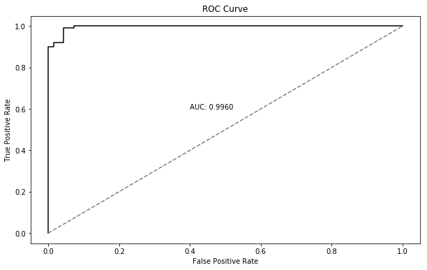
AUC ROC Curve
The models final performance seems quite good, but it’s not really possible to
tell from the above graphs if it’s as good as we can do or not. In particular,
we could be overfitting or underfitting. It also seems to take a long time for
the algorithm to converge (1000 epochs and 3 seconds to converge on just 400
data points in a low-dimensional space? Really?) One powerful diagnostic tool
for evaluating these kinds of problems is to plot both training and validation
loss as a function of iteration. (To do this, it is necessary to instrument
the above code to record these two measurements at the end of every iteration
in the fit() function, but I’ve omitted such details in the code above.)
plt.figure(figsize=(16,6))
plt.ylim(0, 1)
plt.xscale('log')
plt.plot(
    range(1, model.iterations+1),
    model.training_loss_history,
    label='Training Loss')
plt.plot(
    range(1, model.iterations+1),
    model.validation_loss_history,
    label='Validation Loss')
plt.xlabel("iteration")
plt.ylabel("loss-loss")
plt.title("Training/Validation Loss Curve")
plt.legend()
plt.grid(True, 'both')
plt.plot(
    [model.training_loss_history.index(min(model.training_loss_history))],
    [min(model.training_loss_history)],
    marker='o', markersize=7, markerfacecolor='none', color="blue")
plt.plot(
    [model.validation_loss_history.index(min(model.validation_loss_history))],
    [min(model.validation_loss_history)],
    marker='o', markersize=7, markerfacecolor='none', color="orange")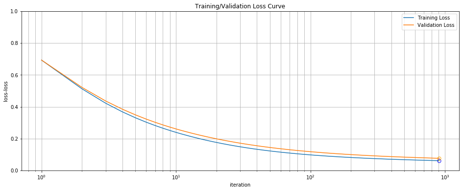
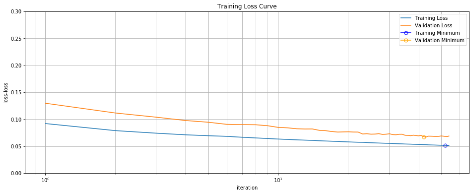
Training/Validation Loss Curve
Note the logarithmic scale used for the x-axis. While we get most of our performance in the first 100 iterations, we continue to make incremental progress up past 1000, at which point we reach our \(10^{-5}\) tolerance for convergence. Because the validation curve also decreases monotonically we at least know we are not overfitting.
So, the batch gradient descent algorithm is finding parameters which minimize training loss to 5 decimal places, which in turn allow it to achieve 97% accuracy on the validation set. There’s no evidence of overfitting. The only real concern is the slow convergence and poor runtime performance. If it takes us 3 seconds to fit 400 data points, how are we going to deal with 400,000 or 40 million? Why is this algorithm so slow, and is there anything we can do about it?
Mini-batch Stochastic Gradient Descent
Stochastic gradient descent may also have properties conceptually similar to simulated annealing which possibly allows it to “jump” out of shallow local minima giving it a better chance of finding a true global minimum. (The concept of a “shallow” vs. “deep” local minimum of a log-likelihood is related to the Cramer-Rao bound which implies that our estimate of parameters \(\hat{\Theta}\) will have less variance under a hypothetical resampling of the training set from the true population if we are at the bottom of a “deep” local minimum with high curvature than if we merely in a “shallow” local minimum with low curvature. This in turn relates to the bias-variance tradeoff in the context of statistical learning theory. Therefore “shallow” minima are bad because if we refit we get very different parameters which increases expected generalization error which is probably the single most meaningful measure of a models performance in real-world scenarios.) Whether or not SGD really has this property or not isn’t something I feel qualified to weigh in on, but it’s a good story, isn’t it?
The reason batch gradient descent is slow is that we evaluate the gradient over the entire training set each time we update the parameters. Not only is this fairly expensive, but it violates a basic principle for making gradient descent algorithm converge rapidly:
Gradients evaluated at a point close to a minima provide more information about the true location of the minima than gradients evaluated far from a minima.
(This principle actually leads to two important optimizations; we’ll see the other shortly.)
A consequence is that if we have the opportunity to take lots of cheap steps instead one expensive step, we should take it. The first step will get us somewhat closer to a minima which makes the later gradient evaluations more valuable.
Because our loss and gradient functions are written as a sum over the rows of some training set, we have a natural way to divide up the work. One approach is to go as far as possible and treat every individual row in the training set as a separate step. This is called stochastic gradient descent. While stochastic gradient descent is fairly stellar early on and can get close to a true minima in just a few minutes, it struggles to converge to an exact value later on when it is close to the final solution. Instead, it can oscillate back and forth around a minima as every row moves it in a contradictory direction. Another issue with SGD is that we can’t really take advantage of vectorization. 10 single row updates can easily take 5 times as long as a single vectorized operation on 10-row matrices.
A good compromise is something called mini-batch gradient descent. We pick a batch size, say between 5 and 100 records each, and partition our training set into as many batches as necessary. It’s OK if some batches are bigger or smaller than the chosen batch size. We do want to ensure that each example is included in one and only one batch, though. It’s also recommended to randomize which examples are placed in which batch every time we pass through the data. The benefits are two-fold: not only are batch steps more likely to in roughly the right direction towards the minima without the back-and-forth pathology of SGD, but we will also get to exploit whatever vectorization primitives our hardware offers. If we’re doing 64-bit floating point arithmetic on an Intel CPU chip with the AVX instruction set, we may see a 4X speed up, for example. The exact benefit, if any should be determined experimentally.
A single pass through all of the batches means that each example in the training set has contributed to the gradient exactly once. We call that one epoch. It should be clear that one epoch requires roughly the equivalent amount of processing as a single iteration of batch gradient descent. Therefore, some of the things we did at the end of each iteration for batch gradient descent, like convergence checking, we will instead do only at the end of each epoch when doing mini-batch stochastic gradient descent.
Leaving all the surrounding code more or less the same, we can implement mini-batch SGD by adding an inner loop inside our fit function.
def fit(self, X, y):
    self.fit_center_scale(X)

    # add intercept column to the design matrix
    n, k = X.shape
    X = self._design_matrix(X)

    # used for the convergence check
    previous_loss = -float('inf')
    self.converged = False

    # initialize parameters
    self.beta = np.zeros(k + (1 if self.add_intercept else 0))
    momentum = self.beta * 0

    for i in range(self.max_iter):
        shuffle = np.random.permutation(len(y))
        X = X[shuffle, :]
        y = y[shuffle]

            # if batch_size does not evenly divide n, we'll one more
            # batch of size less than batch_size at the end.
            runt = (1 if n % self.batch_size else 0)

            for batch_index in range(n // self.batch_size + runt):
                batch_slice = slice(
                    self.batch_size * batch_index,
                self.batch_size * (batch_index + 1) )
            X_batch = X[batch_slice, :]
            y_batch = y[batch_slice]

            y_hat = sigmoid(X_batch @ self.beta)

            # gradient descent
            residuals = (y_hat - y_batch).reshape( (X_batch.shape[0], 1) )
            gradient = (X_batch * residuals).mean(axis=0)
            momentum = 0.8 * momentum + self.learning_rate * gradient
            self.beta -= momentum

        # with minibatch, we only check convergence at the end of every epoch.
        y_hat = sigmoid(X @ self.beta)
        self.loss = np.mean(-y * np.log(y_hat) - (1-y) * np.log(1-y_hat))
        if abs(previous_loss - self.loss) < self.tolerance:
            self.converged = True
            break
        else:
            previous_loss = self.loss

    self.iterations = i+1
Let’s repeat the above tests to see if that improved things:
model = LogisticClassifier(tolerance=1e-5, batch_size=8)
%time model.fit(X_train, y_train)
model.converged, model.iterations, model.loss
CPU times: user 1.36 s, sys: 1.23 s, total: 2.59 s Wall time: 1.31 s
(True, 373, 0.049284666911268454)
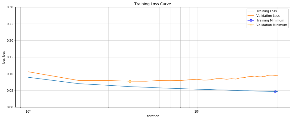
It now takes 1.4 seconds to converge instead of 4 seconds: a 2X wall-clock speed up. It only takes 373 epochs (full passes through the data) instead of the 1,000 for batch gradient descent. And the final result has achieved similar test performance:
Training/Validation Loss Curve Minibatch
Nesterov Accelerated Gradient
But we aren’t even close to done. The next bell-and-whistle on our “Making SGD Awesome” whistle-stop tour is a clever idea called momentum. While there are several competing approaches to implementing momentum, we’ll implement a version called Nesterov Accelerated Gradient.
The basic idea behind momentum is very simple. We want to take the gradient contribution of a given batch and spread it over a number of updates. This is similar to nudging a golf ball in a given direction and allowing it to roll to a stop, hence the name, momentum. How can we achieve this is in a fair way and give the same weight to all batches? By relying on the convergence property of the geometric series. Let’s say we checked the gradient and decided that we wanted to update our parameter \(\Theta\) by a vector \(v = (+2,-2)\). Instead of applying that all in one update, we could apply \(v_0 = (+1,-1)\) the first step, \(v_1 = (+\frac{1}{2}, -\frac{1}{2})\) the second step, \(v_2 = (+\frac{1}{4}, -\frac{1}{4})\) and so on out to infinity. Then by the limit of the geometric series, we know that the total contribution after a long time converges to \((+2,-2)\). More generally, we can choose any decay rate less than one and still enjoy convergence.
\[ \sum_{n=0}^\infty a^n = 1 + a + a^2 + a^3 + ... = \frac{1}{1-a} \,\, \forall a \in \mathbb{R}, 0 \leq a \le 1 \]
That leads to a rule (in pseudocode) like:
momentum = zeros(shape=beta.shape)

for epoch in range(1000):
    for batch in partition_data(X, 8):
        momentum = momentum * decay_rate - learning_rate * gradient(beta, batch)
        beta += momentum
Which is fine, but it turns out we can do strictly better for no extra work if we remember our principle from earlier: gradients taken near a minima are more valuable than those taken further away. In the above pseudocode, we evaluation the gradient at the beta from the previous step, even though we know that part of the update will be to add in the old momentum. So why don’t we do that first and then take the gradient at that point instead? It’s a little bit like peaking ahead.
To help you remember, some mnemonic imagery:
Captain Nesterov stands on the bridge of his submarine. The situation is tense. In the waters above, a Canadian sub-hunter is searching for them. The captain knows that if he can gently land his sub exactly at the lowest point of a nearby indentation in the sea floor, the sub-hunters scan will read them as a natural formation. But if the submarine isn’t at the bottom of the indentation, then they stick out like a sore thumb when the Canadians compare them to their previous topographical survey maps. The captain also knows that he can use at most one ping to measure the depth and angle of the sea floor below them. After that, the sub-hunter will be on high alert and be able to triangulate them on the second ping. Life and death for himself and his entire crew is on the line. The ship glides in silent mode through the inky depths. Nervous, the inexperienced sonar operator cracks. “Do you want me to ping, sir?” “No”, Captain Nesterov replies, “not yet.” the submarine glides on momentum for another tense minute, gradually slowing. Only when the helmsman reports that their speed as dropped another 10% to just 4 knots does he order the ping. By now, the ship has glided to almost the exact center of the depression, and one final course correction sees the ship safely nestled on the sandy ocean floor less than a meter from the lowest point of the depression.
The code for this is straight-forward. Occasionally you’ll see versions of this where the author has bent over backwards to ensure that the prior momentum term is incorporated just once, but this is best left as an exercise for the reader. It has no impact on performance unless a terribly large number of parameters are in play.
def fit(self, X, y):
    self.fit_center_scale(X)

    # add intercept column to the design matrix
    n, k = X.shape
    X = self._design_matrix(X)

    # used for the convergence check
    previous_loss = -float('inf')
    self.converged = False
    self.stopped_early = False

    # initialize parameters
    self.beta = np.zeros(k + (1 if self.add_intercept else 0))
    momentum = self.beta * 0

    for i in range(self.max_iter):
        shuffle = np.random.permutation(len(y))
        X = X[shuffle, :]
        y = y[shuffle]

        # if batch_size does not evenly divide n, we'll one more
        # batch of size less than batch_size at the end.
        runt = (1 if n % self.batch_size else 0)

        for batch_index in range(n // self.batch_size + runt):
            batch_slice = slice(
                self.batch_size * batch_index,
                self.batch_size * (batch_index + 1) )
            X_batch = X[batch_slice, :]
            y_batch = y[batch_slice]

            beta_ahead = self.beta + self.momentum_decay * momentum
            y_hat = sigmoid(X_batch @ beta_ahead)

            # gradient descent
            residuals = (y_hat - y_batch).reshape( (X_batch.shape[0], 1) )
            gradient = (X_batch * residuals).mean(axis=0)
            momentum = self.momentum_decay * momentum - self.learning_rate * gradient
            self.beta += momentum

        # with minibatch, we only check convergence at the end of every epoch.
        y_hat = sigmoid(X @ self.beta)
        self.loss = np.mean(-y * np.log(y_hat) - (1-y) * np.log(1-y_hat))

        if abs(previous_loss - self.loss) < self.tolerance:
            self.converged = True
            break
        else:
            previous_loss = self.loss

    self.iterations = i+1
With our new accelerated momentum, we once again measure performance:
model = LogisticClassifier(
    tolerance=1e-5,
    validation_set=(X_test, y_test))
%time model.fit(X_train, y_train)
model.converged, model.stopped_early, model.iterations, model.loss
CPU times: user 100 ms, sys: 140 ms, total: 240 ms Wall time: 123 ms
(True, False, 30, 0.046659741686488669)
Another simple change to our algorithm, another impressive speed-up. We’re now converging ten times faster than the version without Nesterov Accelerated Momentum, and 25 times faster than the naive batch gradient descent.
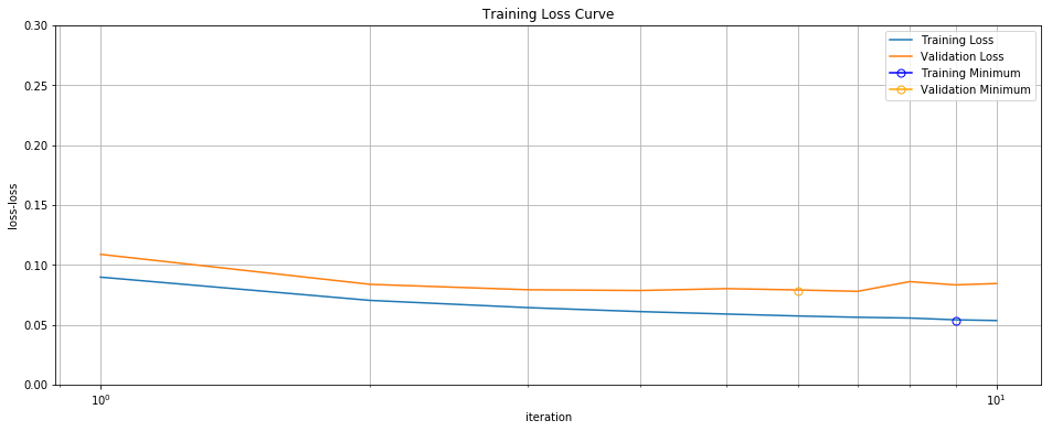
In fact, we’re now converging so fast and efficiently on the training set that a new problem has emerged. Take a look at these loss curves:
Training/Validation Loss Curve
A new phenomenon is occurring: after just a few iterations test set performance first levels off and then actually begins to get worse even as training performance continues to improve. This is actually a classic illustration of the well-known bias-variance trade-off. In fact, the reason we’ve been obsessively recording and plotting training and validation loss for every experiment is because we were on the lookout for the exact phenomenon. And now our caution has paid dividends, because we’ve caught a example of overfitting.
One solution to this kind of overfitting - I mean the kind that gets worse and
worse as the number of iterations increases - is to treat max_iterations as a
hyperparameter and to use a grid search to find the optimal number of
iterations. Or to add regularization, to to play around with batch size, etc.
But there’s a rather clever solution which is as close to a free lunch as
anything I know in machine learning, in the sense that it saves computation
time, minimizes generalization error, and basically costs nothing and has no
downside except for a loss in theoretical rigor. This piece of (black?) magic
is called early stopping.
Early Stopping
The basic idea behind early stopping is taken from looking at the shape of the above validation loss curve. If we want to minimize validation loss, and we know that it goes down for a while then starts to rise, why don’t we just stop once it starts to go back up? Really the only wrinkle is that because the validation loss curve is a little noisy we don’t want to stop the first time we see validation loss rise even a little bit but rather wait to make sure it’s the start of an upward trend before we pull the rip-cord. We can do that simply by waiting for a certain number of epochs with no improvement in validation loss.
One theoretical problem with early stopping is that the parameters estimated in this way are not the maximum likelihood estimates! This makes it harder to reason about them from a statistical point of view. One justification is that although we haven’t found an MLE, we are performing empirical risk minimization and have found a step of parameters that generalize optimally to the validation set. That in turn raises more questions because we haven’t actually minimized empirical risk globally but only along the path of steepest of descent traced out by gradient descent. Ultimately this is a pragmatic technique recommended mainly by its simplicity, improved validation and test set performance, and decreased training times.
Here is the “final” version of the code for the LogisticClassifier, including
implementation details omitted above:
class LogisticClassifier:
    def __init__(self,
            learning_rate=0.1,
            tolerance=1e-4,
            max_iter=1000,
            batch_size=32,
            momentum_decay=0.9,
            early_stopping=3,
            validation_set=(None,None)):
        # gradient descent parameters
        self.learning_rate = float(learning_rate)
        self.tolerance = float(tolerance)
        self.max_iter = int(max_iter)
        self.batch_size=32
        self.momentum_decay = float(momentum_decay)
        self.early_stopping = int(early_stopping)
        self.X_validation, self.y_validation = validation_set

        # how to construct a the design matrix
        self.add_intercept = True
        self.center = True
        self.scale = True

        self.training_loss_history = []

    def _design_matrix(self, X):
        if self.center:
            X = X - self.means
        if self.scale:
            X = X / self.standard_error
        if self.add_intercept:
            X = np.hstack([np.ones((X.shape[0], 1)), X])

        return X

    def fit_center_scale(self, X):
        self.means = X.mean(axis=0)
        self.standard_error = np.std(X, axis=0)

    def fit(self, X, y):
        self.fit_center_scale(X)

        # add intercept column to the design matrix
        n, k = X.shape
        X = self._design_matrix(X)

        # used for the convergence check
        previous_loss = -float('inf')
        self.converged = False
        self.stopped_early = False

        # initialize parameters
        self.beta = np.zeros(k + (1 if self.add_intercept else 0))
        momentum = self.beta * 0  # trick to get the same shape and dtype as beta

        for i in range(self.max_iter):
            shuffle = np.random.permutation(len(y))
            X = X[shuffle, :]
            y = y[shuffle]

            # if batch_size does not evenly divide n, we'll one more
            # batch of size less than batch_size at the end.
            runt = (1 if n % self.batch_size else 0)

            # if batch_size does not evenly divide n, we'll one more
            # batch of size less than batch_size at the end.
            runt = (1 if n % self.batch_size else 0)

            for batch_index in range(n // self.batch_size + runt):
                batch_slice = slice(
                    self.batch_size * batch_index,
                    self.batch_size * (batch_index + 1) )
                X_batch = X[batch_slice, :]
                y_batch = y[batch_slice]

                beta_ahead = self.beta + self.momentum_decay * momentum
                y_hat = sigmoid(X_batch @ beta_ahead)

                # gradient descent
                residuals = (y_hat - y_batch).reshape( (X_batch.shape[0], 1) )
                gradient = (X_batch * residuals).mean(axis=0)
                momentum = self.momentum_decay * momentum - self.learning_rate * gradient
                self.beta += momentum

            # with minibatch, we only check convergence at the end of every epoch.
            y_hat = sigmoid(X @ self.beta)
            self.loss = np.mean(-y * np.log(y_hat) - (1-y) * np.log(1-y_hat))
            self.training_loss_history.append(self.loss)

            # early stopping
            if self.check_validation_loss():
                self.stopped_early = True
                break

            if abs(previous_loss - self.loss) < self.tolerance:
                self.converged = True
                break
            else:
                previous_loss = self.loss

        self.iterations = i+1

    def predict_proba(self, X):
        # add intercept column to the design matrix
        X = self._design_matrix(X)
        return sigmoid(X @ self.beta)

    def predict(self, X):
        return (self.predict_proba(X) > 0.5).astype(int)

    def check_validation_loss(self):
        # validation set loss
        if not hasattr(self, 'validation_loss_history'):
            self.validation_loss_history = []
        p_hat = self.predict_proba(self.X_validation)
        loss = np.mean(-self.y_validation * np.log(p_hat) - \
               (1-self.y_validation) * np.log(1-p_hat))
        self.validation_loss_history.append(loss)

        # AUC ROC history
        if not hasattr(self, 'auc_history'):
            self.auc_history = []
        auc = roc_auc_score(self.y_validation, p_hat)
        self.auc_history.append(auc)

        t = self.early_stopping
        if t and len(self.validation_loss_history) > t * 2:
            recent_best = min(self.validation_loss_history[-t:])
            previous_best = min(self.validation_loss_history[:-t])
            if recent_best > previous_best:
                return True
        return False
OK, one last time: how’s the performance?
model = LogisticClassifier(
    tolerance=1e-5,
    early_stopping=3,
    validation_set=(X_test, y_test))
%time model.fit(X_train, y_train)
model.converged, model.stopped_early, model.iterations, model.loss
CPU times: user 40 ms, sys: 30 ms, total: 70 ms Wall time: 49.1 ms (False, True, 10, 0.053536116001088603)
Convergence is crazy fast. 49 ms? Is that some kind of joke? We started with 3 seconds and now you’re telling me its 49 ms? As in, 60X faster? No, this is actually fairly typical. That’s why it’s so important to use a good optimizer instead of relying on naive methods. Luckily, with modern frameworks, state-of-the-art optimizers are usually available off-the-rack.
Test set performance (accuracy, AUC) has not suffered:

AUC ROC Curve
The loss curves are exactly the same as before… until the curve starts climbing upward for a few iterations, at which point we pull the plug. In this case, we stopped after just 10 iterations, compared to the 1000 needed for the batch gradient descent.
Training/Validation Loss Curve
Conclusion
That was logistic regression from scratch. In this article, we’ve learned about a simple but powerful classifier called logistic regression. We derived the equations for MLE and, in our attempts to solve these equations numerically, developed an incredibly powerful piece of technology: Mini-batch SGD with early stopping and NAG. This optimizer is actually more important than logistic regression because it turns out it can be re-used for a wide variety of models.
There are variations on SGD that we haven’t talked about, in particular
adaptive variations which don’t need a learning_rate hyperparameter or have
schedules for changing learning_rateor momentum_decay over time. But
there’s no general, one-size-fits-all solution which is strictly better than
the technique presented here. You will of course find endless papers and
benchmarks suggesting that one technique or another is better; but they’re
are generally talking about differences less that 2X, not the 60X gained
by these more fundamental techniques.
I myself often use Adam as my go-to optimizer on new datasets, simply because it works even when the data isn’t centered and scaled and I don’t have to fiddle around with learning rate. The idea isn’t to argue that this particular algorithm is the best choice for all possible scenarios - no such algorithm exists. But hopefully we’ve covered the key ingredients which go into a state-of-the-art optimizer.
In the next installment of Machine Learning From Scratch, we’ll explore neural networks and the backpropagation algorithm in particular.