Complex Numbers in R, Part II

Complex Roots and Eigenvalues

Some problems are specific to complex numbers, some problems can be made easier by a complex representation, and some problems have complex numbers thrust upon them.

– William Shakespeare, 12 + 5i Night

One such case that is of interest to statisticians and scientists (I’m assuming you’re not using R for embedded systems or game development) is solving the eignproblem for a non-symmetric matrix.

Now, if your only exposure to eigenvalues is through PCA, you might not even be aware that eigenvalues are usually complex numbers… even when the original matrix is comprised only of real numbers! However PCA is actually a very special case: a covariance matrix is always a symmetric, positive-definite, real-valued matrix, therefore its eigenvalues are always positive real numbers.

However, there are plenty of situations in statistics where a non-symmetric matrix arises naturally and the eigenvalues can give us deep insight into the problem. Two such are Markov Chains and AR models. Let’s only look at a simple example of an AR model - that will suffice to demonstrate R’s complex number functionality in this domain.

Let’s start by constructing a small time series that exhibits very strong autocorrelation. To get some interesting behavior, I will give it a strongly positive one day correlation, but then reverse it the next day. This should give us both decay and oscillations.

set.seed(43)
t_0 <- zoo(rnorm(n=100))
t_1 <- lag(t_0, k=1, na.pad=TRUE)
t_2 <- lag(t_0, k=2, na.pad=TRUE)
t_3 <- lag(t_0, k=3, na.pad=TRUE)
t <- na.omit(t_0 + 0.7*t_1 - 0.2*t_2 + 0.2*t_3)
plot(t, type='l')
title('Time Series With Autocorrelation')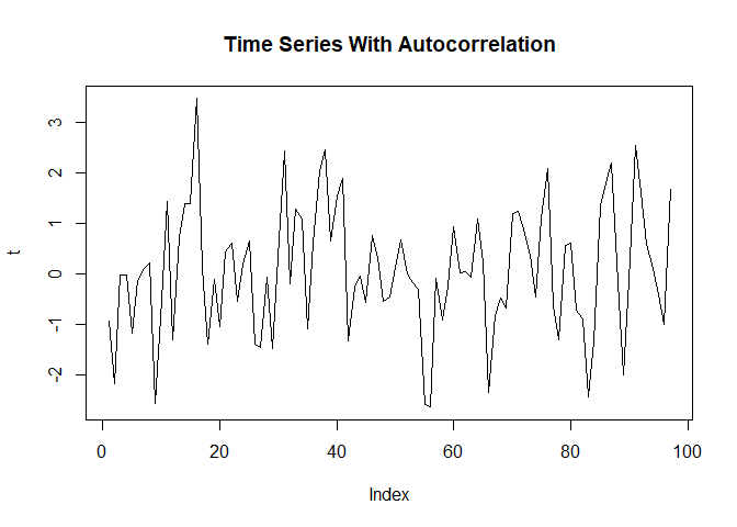

pacf(t) # Partial Autocorrelation Plot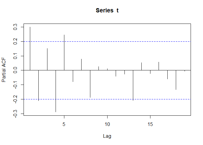

Next we construct the model. While I normally recommend the forecast package, we’ll just use the built-in ar() function today.

ar_model <- ar(t)
ar_model

# 
# Call:
# ar(x = t)
# 
# Coefficients:
#       1        2        3        4        5  
#  0.5078  -0.4062   0.3481  -0.3960   0.2462  
# 
# Order selected 5  sigma^2 estimated as  1.19

That’s roughly what we’d expect based on how we constructed the time series and what we saw on the partial autocorrelation plot: A strong positive autocorrelation at lag one, a slightly less strong negative autocorrelation at lag 2, then some harmonics.

ar_coefs <- ar_model$ar  # coefficients(ar_model) doesn't work, IDK why
roots <- polyroot( c(1,-ar_coefs) )
roots

# [1]  0.7158218+1.1364815i -0.6823253+0.9974625i -0.6823253-0.9974625i
# [4]  0.7158218-1.1364815i  1.5417367+0.0000000i

plot(
  1/roots, 
  ylim=c(-1,1), 
  asp=1,
  main="Inverse AR Roots",
  panel.first=c(
    lines(complex(modulus=1, argument=0.01*2*pi)^(0:100), col='grey'),
    abline(h=0, col='grey'),
    abline(v=0, col='grey')
  )
)

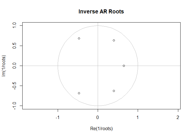
Just to be clear, we’re plotting the inverse roots, so we’d expect them to be inside the unit circle if the process is stationary.

(Just as an Easter egg, we also used complex numbers to plot the unit circle. If you’re not sure how that worked, just remember that multiplying complex numbers adds their arguments – their angle with the x-axis – together.)

Just from looking at the roots and observing that some are far from the real axis, we can also say that this time series will experience a back-and-forth oscillations as each day tries to “correct” for the previous day. If the influence of history merely decayed away smoothly and exponentially, all the roots would have been close to the real axis. (It’s a common misconception that how long effects last is related to the order of the model; when in fact even an AR(1) model can have a very long memory if it has its root close to 1.)

Plotting the inverse roots of ARIMA models is standard practice because it can help you diagnose non-stationary series and near unit roots, both of which can ruin the predictive power and interpretability of a model. There’s no getting away from the fact that a polynomial of degree two or higher might have complex roots.

But there’s another way of looking at an AR model - as a discrete linear dynamical system. Let’s call the value of our at the \(n\)-th step \(t_n\). Then we can define our state vectors to be

\[ \boldsymbol{t}_n = \begin{bmatrix} t_n \\ t_{n-1} \\ t_{n-2} \\ t_{n-3} \\ t_{n-4} \\ \end{bmatrix} \]

In other words, we just stack \(t_n\) with it’s first four lags. That may not seem like an improvement, but now we can write

\[ \boldsymbol{t}_{n+1} =\boldsymbol{F} \boldsymbol{t}_n \]

or more explicitly:

\[ \begin{bmatrix} t_{n+1} \\ t_{n} \\ t_{n-1} \\ t_{n-2} \\ t_{n-3} \\ \end{bmatrix} = \boldsymbol{F} \begin{bmatrix} t_n \\ t_{n-1} \\ t_{n-2} \\ t_{n-3} \\ t_{n-4} \\ \end{bmatrix} \]

where \(\boldsymbol{F}\) is the “forward time evolution” matrix. This basically says we can always compute the state of our time series at the next time step by applying a linear operator to the previous state. And in fact, we already have a good idea what the matrix \(\boldsymbol{F}\) should look like. For one thing, it’s clear that the four lagged components can simply be grabbed from the old state by shifting down by one:

\[ \begin{bmatrix} t_{n+1} \\ t_{n} \\ t_{n-1} \\ t_{n-2} \\ t_{n-3} \\ \end{bmatrix} = \begin{bmatrix} . & . & . & . & . \\ 1 & 0 & 0 & 0 & 0 \\ 0 & 1 & 0 & 0 & 0 \\ 0 & 0 & 1 & 0 & 0 \\ 0 & 0 & 0 & 1 & 0 \\ \end{bmatrix} \begin{bmatrix} t_n \\ t_{n-1} \\ t_{n-2} \\ t_{n-3} \\ t_{n-4} \\ \end{bmatrix} \]

And from the coefficients of the AR(1) model we built before, we know that \(t_n\) can be expressed as a linear sum of \(t_{n-1}\) through \(t_{n-4}\):

\[ \begin{bmatrix} t_{n+1} \\ t_{n} \\ t_{n-1} \\ t_{n-2} \\ t_{n-3} \\ \end{bmatrix} = \begin{bmatrix} 0.508 & -0.406 & 0.348 & -0.396 & 0.246 \\ 1 & 0 & 0 & 0 & 0 \\ 0 & 1 & 0 & 0 & 0 \\ 0 & 0 & 1 & 0 & 0 \\ 0 & 0 & 0 & 1 & 0 \\ \end{bmatrix} \begin{bmatrix} t_n \\ t_{n-1} \\ t_{n-2} \\ t_{n-3} \\ t_{n-4} \\ \end{bmatrix} \]

So now that, we’ve determined the linear operator \(\boldsymbol{F}\) for our dynamic system, we can ask what happens to the system 2 time-steps into the future, then 3, and so on. It should be clear that we can simply apply \(\boldsymbol{F}\) again and again to determine any future state, so that in general the state at time \(n\) is

\[ \boldsymbol{t}_n = \boldsymbol{F}^n \boldsymbol{t}_0 \]

But raising a matrix to a power is particularly easy if we know its eigenvalues. Let’s say \(\boldsymbol{F} = \boldsymbol{Q} \boldsymbol{\Lambda} \boldsymbol{Q}^{-1}\) is the eigen-decomposition, where \(\boldsymbol{Q}\) is an orthogonal matrix and \(\boldsymbol{\Lambda}\) is the diagonal matrix of eigenvalues. Then

\[ \boldsymbol{F}^2 = \boldsymbol{F} \boldsymbol{F} = \boldsymbol{Q} \boldsymbol{\Lambda} \boldsymbol{Q}^{-1} \boldsymbol{Q} \boldsymbol{\Lambda} \boldsymbol{Q}^{-1} = \boldsymbol{Q} \boldsymbol{\Lambda}^2 \boldsymbol{Q}^{-1} \]

This clearly generalizes to any power by induction. Also, raising a diagonal matrix to a power is completely trivial: you simply raise each independent element to its power.

\[ \boldsymbol{\Lambda}^n = \begin{bmatrix} \lambda_1^n & 0 & 0 & 0 & 0 \\ 0 & \lambda_2^n & 0 & 0 & 0 \\ 0 & 0 & \lambda_3^n & 0 & 0 \\ 0 & 0 & 0 & \lambda_4^n & 0 \\ 0 & 0 & 0 & 0 & \lambda_5^n \end{bmatrix} \]

A few things are immediately obvious. Each eigenvalue is a complex number; so if its norm is less than 1 it will tend to 0 as \(n\) increases, or if its norm is greater than 1 it will tend to \(\infty\), or if its norm is exactly 1 it will always be exactly 1. Furthermore, if the eigenvalue is real, it will always be real, but if it is not real then it will rotate about the origin by a fixed angle with every time step. Thus, it will exhibit some kind of oscillation with a frequency determined by its argument. Each eigenvalue will behave independently, but if every eigenvalue has norm less than 1, then the system as a whole will converge to a steady state at 0.

So now that I’ve hopefully impressed upon you the importance of eigenvalues is understanding the dynamics of our system, let’s actually compute them. And, just for fun let’s compare them to the roots of the lag polynomial from above.

ar_matrix <- matrix( nrow=5, ncol=5, byrow=TRUE, c(
  0.5078, -0.4062,   0.3481,  -0.3960,   0.2462, 
       1,       0,        0,        0,        0,
       0,       1,        0,        0,        0,
       0,       0,        1,        0,        0,
       0,       0,        0,        1,        0))

ar_eigen <- eigen(ar_matrix)
df <- t(rbind(
  data.frame(t(sort(1/roots))), 
  data.frame(t(sort(ar_eigen$values)))))
colnames(df) <- c("Inverse AR(5) Roots", "Time Evolution Eigenvalues")

Inverse AR(5) Roots	Time Evolution Eigenvalues
-0.467 + 0.683i	-0.467 - 0.683i
-0.467 - 0.683i	-0.467 + 0.683i
0.397 + 0.630i	0.397 - 0.630i
0.397 - 0.630i	0.397 + 0.630i
0.649 - 0.000i	0.649 + 0.000i

Hey, wait just a minute here! What are you trying to pull here, buddy? Those are (to within numerical precision) exactly the same as the inverse roots!

Yes, it’s true. This is very obvious if we plot them together:

plot(
  ar_eigen$values, 
  ylim=c(-1,1), 
  xlim=c(-1,1),
  asp=1,
  cex=2,
  main="Inverse AR Roots",
  panel.first=c(
    lines(complex(modulus=1, argument=0.01*2*pi)^(0:100), col='grey'),
    abline(h=0, col='grey'),
    abline(v=0, col='grey')
  )
)

points(
  1/roots, 
  pch=4,
  cex=2,
  col='red'
)

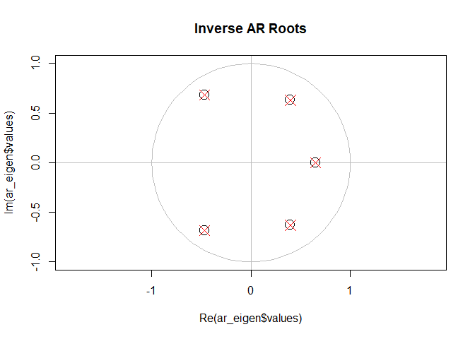
They are exactly the same. You’re welcome to prove this for yourself by writing down the characteristic polynomial for a matrix in this form and verifying it’s the exact same polynomial we found the roots for in the AR formulation of the problem.

In fact, you can see the many parallels in the two approaches: in one analysis, we said that an AR model would only be stationary if all its inverse roots were inside the unit circle, in the other we said the dynamic system would converge to a steady state at the origin. Different language, indeed two historically different mathematical treatments, but the same conclusions. In both cases we found that the system was characterized by a sequence of 5 complex numbers, and that both the norm and the argument of each number meaningfully impacted the behavior of the system. And so on.

There’s no escaping it: those 5 complex numbers are the best way to understand this system, and any sufficiently sophisticated approach will lead us to this same conclusion.

Let’s just take a moment to realize what happened to us here: we started from a data set entirely comprised of real numbers, built a model with real number values for all parameters but in the end we still had to understand our model in terms of complex numbers.

The hard truth is that the real numbers are not closed under many interesting and natural operations… if you work with real numbers long enough, you’ll eventually find yourself in the complex plane.

Luckily, R really does have excellent support for complex numbers – if nothing else, I hope I’ve familiarized you with some of that functionality.