
Adaptive Basis Functions
Today, let me be vague. No statistics, no algorithms, no proofs. Instead, we’re going to go through a series of examples and eyeball a suggestive series of charts, which will imply a certain conclusion, without actually proving anything; but which will, I hope, provide useful intuition.
The premise is this:
For any given problem, there exists learned featured representations which are better than any fixed/human-engineered set of features, even once the cost of the added parameters necessary to also learn the new features into account.
This is of course completely unoriginal: it is in in fact the standard just-so story for machine learning that you hear again and again in different contexts. The learned \(k \times k\) kernels of a 2D CNN works better than Haar features or Sobel filters. A one dimensional CNN and a spectrogram works better than MFCC. An ensemble of decision stumps works better than a single large decision tree. And so on.
Even as mythology, there are already plenty of cracks starting to show. The biggest and most well known caveat is of course, “given a sufficiently huge amount of training data.” There are often other caveats too, such as “and you don’t care how slow it is.” For example, the Viola-Jones object detection framework uses Haar features and is still widely used because it is so much faster than CNN-based approaches, although not as robust or accurate. While cutting edge CNN-based object detectors are starting to achieve acceptable runtime performance, they’ll probably never be as fast as Haar features, simply because they’ll never be able to take advantage of the integral image trick.
But let’s zoom out at look at the big picture instead of shopping around for counterexamples and limitations. At a high level, the story is clear. Again and again, on various problems and algorithms, we’ve seen that taking carefully engineered representations, often with very attractive mathematical properties which make them tractable for computation and mathematical analysis, and just throwing them out to start over from scratch with a learned representation is a winning strategy. It not only works, it often smashes straight through the performance ceiling where the previous generation of models had plateaued. The history of the ImageNet challenge provides plenty of concrete examples of that.
But these successes are on very large and complicated problems; is it possible to find a simpler example of the phenomenon, so that a student can actually wrap their head around it? Or does the phenomenon only manifest once the problem hits a certain threshold of complexity? I think it is possible to find such elementary problems that demonstrate the power of learned representations.
Once such example, which happily lends itself to easy visualization, is the problem of learning to approximate a one-dimensional function. To make the case in favor of learned representations we will first attempt the problem with several fixed representations and compare those attempts with a learned representation.
The Function Approximation Problem
Given an i.i.d. random sample \(\{(Y_i, X_i)\}_{i=1}^n\) where \(X\) and \(Y\) have joint probability distribution \(F\), we wish to find a real-valued function \(f : \mathbb{R} \mapsto \mathbb{R}\) such that:
\[ E[Y|X] = f(x) \]
Since we only have access to the random sample, we cannot hope to find an exact solution, but can find the best (in terms of MSE) function from some family of functions \(\mathcal{F}\):
\[ \hat{f} = \underset{f \in \mathcal{F} }{{\text{argmin}}} \sum_i^n (f(x) - E[Y|X])^2 \tag{1} \]
The question then becomes how we choose a family \(\mathcal{F}\) that makes this optimization problem tractable. The obvious answer is to parameterize \(\mathcal{F}\) in terms of \(k\) real-valued parameters; then the optimization problem is to find the minimum of the loss function \(J : \mathbb{R}^k \mapsto \mathbb{R}\) which can be solved with standard techniques.
The standard way to define such a parameterization is to assume that \(f\) is the weighted sum of \(k\) fixed basis functions \(\psi_1, ..., \psi_k\) and let \(\mathcal{F} = \text{span} \{ \psi_1, ..., \psi_k \}\). Then, for any function \(f \in \mathcal{F}\), we can always write \(f\) as a linear combination of basis functions:
\[ f(x) = \sum_{i=j}^k \beta_j \psi_j(x) \tag{2} \]
Substituting (2) into (1) above, we have an explicit loss function:
\[ J(\beta) = \sum_{i=1}^n (E[Y|X] - \sum_{j=1}{k} \beta_j \psi_j(x) )^2 \tag{3} \]
When \(J\) is as small as possible, \(\hat{f}\) is as close as possible to the target function \(f\) as it is possible for any function in \(V\) to be. We say that \(\hat{f}\) is the best approximation of \(f\) for the given choice of basis functions \(\psi_1, ..., \psi_N\).
We will call the choice of parameters that minimize loss \(\hat{\beta}\) and the corresponding function \(\hat{f}\):
\[ \begin{align} \hat{\beta} & = \text{argmin}_\beta J(\mathbf{\beta}) \tag{4} \\ \hat{f}(x) & = \sum_{j=1}^k \hat{\beta}_j \psi_j(x) \tag{5} \end{align} \]
We won’t dwell too much today on the best way to actually solve this minimization problem but instead just use an off-the-shelf solver to quickly (in terms of programmer time) get a workable solution. Instead, we’ll focus on how the choice of basis functions affects our ability to approximate a function.
Target Function
For the examples below, we’re going to need some target function \(t(x) = E[Y|X]\). It should be continuous, bounded on some closed interval, and it’s also convenient if it’s approximately zero on both edges. The unit interval \([0, 1]\) is as good a choice for the domain as any. To make the function appropriately ugly, we’ll take some polynomial terms plus some sinusoidal terms: that will make it hard to approximate with either Fourier series or a splines, and also give us lots of nasty inflections.
import matplotlib
import matplotlib.pyplot as plt
%matplotlib inline
import numpy as np
import math
np.warnings.filterwarnings('ignore')
from scipy.optimize import minimize

def target_function(x):
    return x*(x-1) * (np.sin(13*x) + np.cos(23*x)*(1-x))
x = np.linspace(start=0, stop=1, num=101)
y = target_function(x) #+ np.random.normal(0, 0.1, size=x.shape)

plt.figure(figsize=(16,10))
plt.title("Arbitrary Smooth Function")
plt.plot(x, y, label="target")
plt.legend()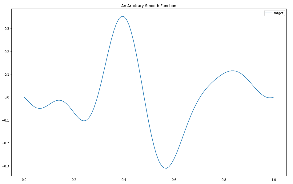
Target Function
I wouldn’t say this function is pathological, but it’s juuust hard enough to be interesting.
Step Function Basis
To get warmed up, let’s use the above basis function framework to calculate the best possible step function approximation of a function. Since our target function is continuous this approach if fundamentally flawed but it illustrates the method.
First, we will define a finite set of fixed basis functions:
N_step = 20

def step_function(i):
    return lambda x: np.where(x > i/N_step, 1, 0)

def sum_of_step_functions(beta):
    def f(x):
        total = np.zeros(shape=x.shape)
        for i, b in enumerate(beta):
            total += step_function(i)(x) * b
        return total
    return f

def square_function_distance(f, g):
    return np.sum( (f(x) - g(x))**2 )

def step_loss(beta):
    g = sum_of_step_functions(beta)
    return square_function_distance(target_function, g)

plt.figure(figsize=(16,10))
plt.title("Step Function Basis")
for i in range(N_step):
    plt.plot(x, step_function(i)(x))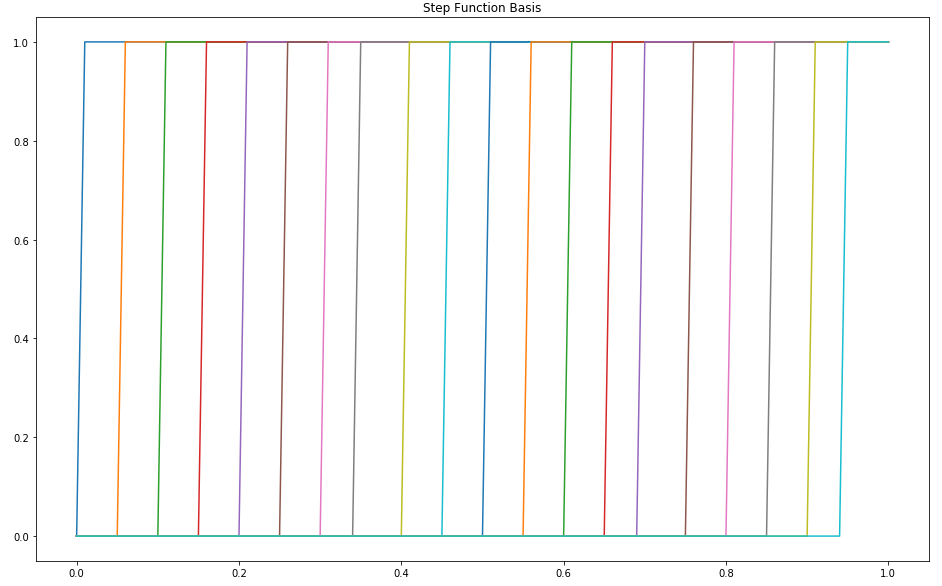
Step Basis
In this case, each basis function is a step function and the only difference between them is the position at which the step occurs.
To construct our approximation, we choose the best coefficient for each basis function:
best = minimize(step_loss, x0=np.zeros(shape=N_step))
beta_hat = best.x
if best.status != 0:
print(best.message)
plt.figure(figsize=(16,10))
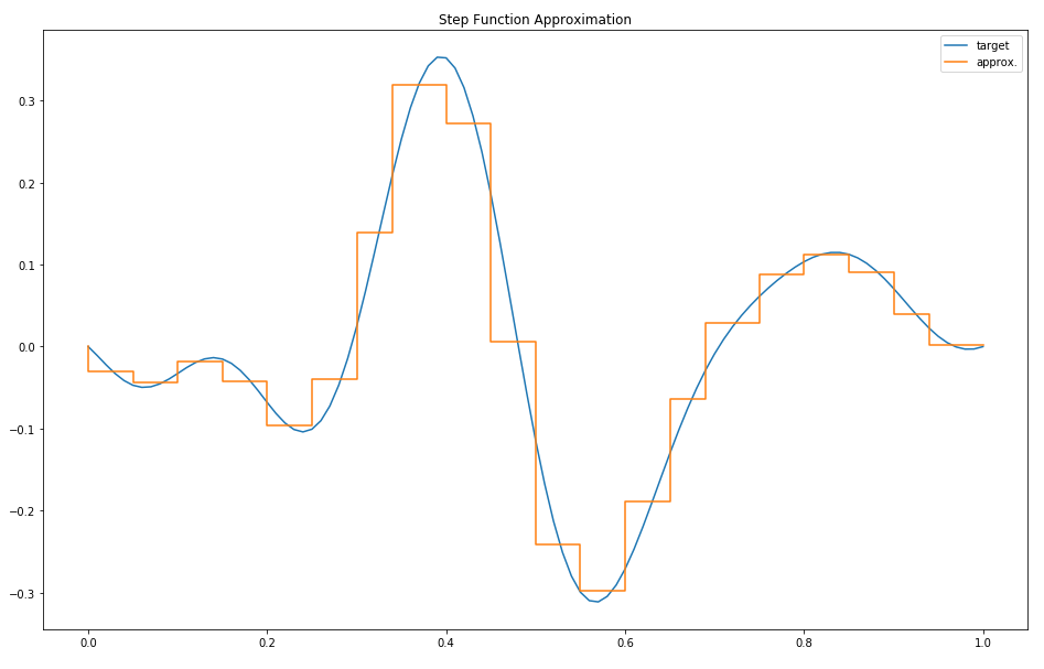
plt.title("Step Function Approximation")
plt.plot(x, y, label='target')
plt.step(x, sum_of_step_functions(beta_hat)(x), label='approx.')
plt.legend()
print("best loss:", step_loss(beta_hat))best loss: 0.1127449592291812
Unsurprisingly, this approximation is able to get reasonably close on each small interval but is ultimately hampered by its inability to represent slopes.
Step Approximation
Fixed Sigmoid Basis Functions
Since we know our target function is continuous, it makes sense to likewise choose continuous basis functions. Since the step function otherwise seem to have worked reasonably well, we’ll simply use a smoothed version of the step function, the so-called sigmoid function.
def sigmoid_basis_function(i):
    return lambda x: 1/(1+np.exp((i- 10*x)/1.73))

def sum_of_sigmoid_functions(beta):
    def f(x):
        total = np.zeros(shape=x.shape)
        for i, b in enumerate(beta):
            total += sigmoid_basis_function(i)(x) * b
        return total
    return f

def sigmoid_loss(beta):
    g = sum_of_sigmoid_functions(beta)
    return square_function_distance(target_function, g)

plt.figure(figsize=(16,10))
plt.title("Fixed Sigmoid Basis")
for i in range(10):
    plt.plot(x, sigmoid_basis_function(i)(x))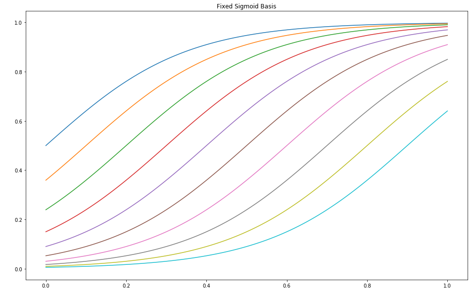
Sigmoid Basis
Note that the functions in this basis are only distinguished by their offset.
best = minimize(sigmoid_loss, x0=np.zeros(shape=10))
beta_hat = best.x
if best.status != 0:
print(best.message)
plt.figure(figsize=(16,10))
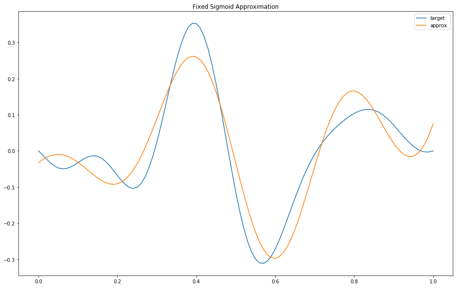
plt.title("Fixed Sigmoid Approximation")
plt.plot(x, y, label="target")
plt.plot(x, sum_of_sigmoid_functions(beta_hat)(x), label="approx.")
plt.legend()
print("best loss:", sigmoid_loss(beta_hat))best loss: 0.2857660082499814
Sigmoid Approximation
While more visually appealing, this hasn’t really done better than the step function basis.
Orthogonal Basis Functions
Families of orthogonal functions have a key property that makes them especially useful as basis functions: you can determine the optimal coefficient \(\beta_j\) without considering any of the other elements of \(\mathbf{\beta}\).
The Fourier series is one well-known example. The basis functions are \(sin(nx)\) and \(cos(nx)\) for \(n>0\) plus the constant function.
def fourier_basis_function(i):
    if i == 0:
        return lambda x: np.full_like(x, 0.5)
    else:
        n = (i+1)//2
        if i % 2 == 1:
            return lambda x: np.sin(n*x)
        else:
            return lambda x: np.cos(n*x)

def sum_of_fourier_functions(beta):
    def f(x):
        total = np.zeros(shape=x.shape)
        for i, b in enumerate(beta):
            total += fourier_basis_function(i)(x) * b
        return total
    return f

def fourier_loss(beta):
    g = sum_of_fourier_functions(beta)
    return square_function_distance(target_function, g)

plt.figure(figsize=(16,10))
plt.title("Fourier Basis")
for i in range(5):
    theta = x * 2 * math.pi
    plt.plot(theta, fourier_basis_function(i)(theta))
plt.axhline(y=0, color='k', linewidth=1)
There are faster ways to compute the coefficients in the particular case of the Fourier series, but we’ll just brute force like always for consistencies sake.
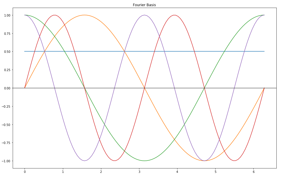
Fourier Basis
best = minimize(fourier_loss, x0=np.zeros(shape=21))
beta_hat = best.x
if best.status != 0:
    print(best.message)

plt.figure(figsize=(16,10))
plt.title("Fourier Approximation")
plt.plot(x, y, label="target")
plt.plot(x, sum_of_fourier_functions(beta_hat)(x), label="approx.")
plt.legend()
print("best loss:", fourier_loss(beta_hat))
best loss: 0.15528347938817644
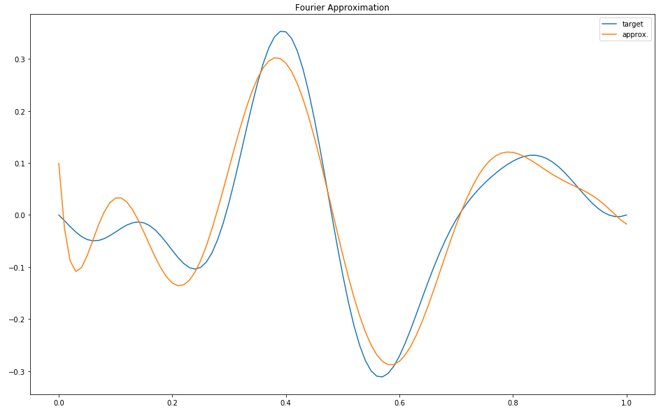
Fourier Approximation
The fit isn’t particularly great, even using 21 parameters, which is equivalent to adding up ten sine waves each with different amplitudes and frequencies. That’s to be expected: Fourier series are pretty bad at approximating polynomials, and are even worse at approximating functions with discontinuities.
An orthogonal family of basis functions can work really well when they are well suited to your problem – for example, when the target function is known to be solution to some differential equation, and each basis function is likewise a solution to that same differential equation. But they are often a very poor choice when we know little about the target function.
While there might be a theoretical guarantee that we can approximate any function given an unlimited number of Fourier basis functions, this can require an unreasonably large number of parameters before a good fit is achieved. But every parameter we add to the model increases our chances of overfitting! We need to look for a way of approximating functions well while keeping the number of parameters under control.
Adaptive Basis Functions
Finally, we come to our ringer: the adaptive basis function. Within the context of function approximation, adaptive basis functions are a clear example of a learned representation. Kevin Murphy’s book has a good chapter on adaptive basis function models, but a very simple working definition is that they are models where the basis functions themselves are parameterized, and not just the weights out front.
The way to ensure that each basis function added to the model is adding value and isn’t just dead weight is to give each basis function its own parameters, which we will learn in parallel with the coefficients. Note that this means we are leaving the additive assumption behind. While the model may still superficially look like an additive model:
\[ f(x) = \sum_{i=j}^N \beta_j \psi_j(x;\theta_j) \]
Each \(\psi_j\) is now a parameterized function rather than a fixed basis function. This makes computing gradients much harder, and almost always means that the new optimization problem is no longer convex.
There is also a trade-off in the number of parameters used: while we have fewer \(\beta_j\) parameters, we also have new \(\theta_j\) parameters. Hopefully there will be some sweet spot where each adaptive basis function is doing the work of many fixed basis functions!
A good choice for adaptive basis functions is the sigmoid. We can add parameters that shift it left or right, make it wider or narrower:
def learned_basis_function(bias, width):
    return lambda x: 1/(1+np.exp((bias - x)/width))

def sum_of_learned_functions(beta):
    beta = beta.reshape( (beta.size//3,3) )
    def f(x):
        total = np.zeros(shape=x.shape)
        for i, b in enumerate(beta):
            total += learned_basis_function(b[1], b[2])(x) * b[0]
        return total
    return f

def learned_basis_loss(beta):
    g = sum_of_learned_functions(beta)
    return square_function_distance(target_function, g)

plt.figure(figsize=(16,10))
plt.title("Learned Sigmoid Basis")
for i in [1, 3, 5, 7, 9]:
    bias = i/10
    for width in [0.1, 0.2, 0.3]:
        plt.plot(x, learned_basis_function(bias, width)(x))
Here is only a small sample of what is possible with these basis functions. In fact, there are infinitely many possible adaptive sigmoid functions - although we will be forced to choose just a small number (\(k=7\) below) to construct our approximation.
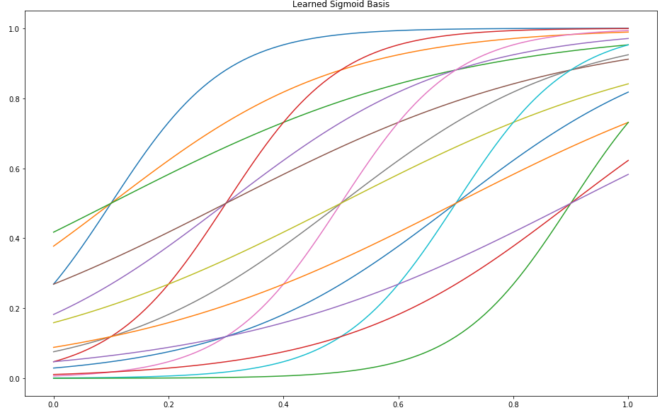
Learned Sigmoid Basis
Note that a very narrow sigmoid is basically a step function, while a very wide sigmoid is basically linear! It’s like we’re getting a two-for-one deal - the space of possible functions \(\mathcal{F}\) now includes the span of the sum of all possible step functions and all possible linear functions, as well as all the smooth sigmoid functions in between. This is a very robust representation that should be able to model very complex real-world relationships.
Also note that \(k=7\) is not quite arbitrary – because we have 3 parameters per adaptive basis function, this is roughly the same number of parameters as the above examples. At first it may seem like that’s not nearly enough. Recall that 7 fixed sigmoid functions did a very poor job! But remember, these are adaptive. During training, each of the seven can be shifted and scaled independently of the others. This allows the model to move each to the perfect place where it can do the most good.
k = 7
best_loss = float('inf')
beta_hat = np.zeros( shape=(k, 3) )
for iteration in range(10):
    beta_zero = np.random.normal(0, 0.01, size=(k,3))
    beta_zero[:, 1] = np.linspace(0, 1, k)
    beta_zero[:, 2] = np.ones(shape=k) * 0.2
    print('fitting attempt', iteration)
    best = minimize(learned_basis_loss, x0=beta_zero)
    candidate_beta = best.x.reshape( (k,3) )
    candidate_loss = learned_basis_loss(candidate_beta)
    if candidate_loss < best_loss:
        best_loss = candidate_loss
        beta_hat = candidate_beta

print('beta:', beta_hat)
print("best loss:", learned_basis_loss(beta_hat))
if best.status != 0:
    print(best.message)
best loss: 0.00012518241681862751
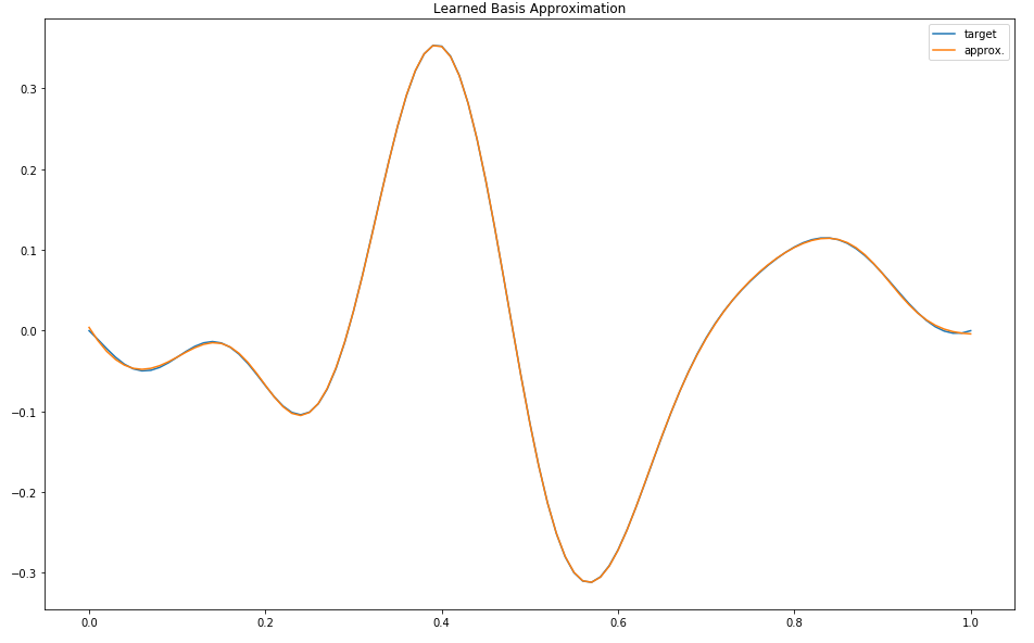
Learned Sigmoid Approximation
OK, that went from zero to sixty pretty quickly. This is so absurdly good that you have to squint to even see, yes, the blue line for the target is still there, it’s just mostly covered by the orange line for the approximation. We’re using roughly the same number of parameters as before, so why is this so much better?
The only answer that I can give you is that adaptive basis functions are an example of a learned representation, and that by picking (learning) 7 basis functions that were “perfect” for this specific problem, we can build a much better model with just a handful of them.
But here’s the punchline: this representation – a linear combination of adaptive sigmoid functions – is exactly the same as a neural network with one hidden layer.
In particular, a neural network with one input node, one hidden layer with a sigmoid activation function, and one output node with a linear activation function. In diagram form for \(k = 7\), each of the 21 gray connection lines corresponds to exactly one of the parameters of the model:
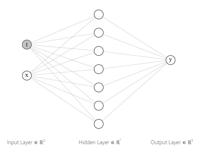
Neural Network Architecture
(Astute readers may notice a missing bias node on the hidden layer; that is because the above implementation does not in fact have a corresponding parameter. But is is a completely inconsequential difference and could have been easily added to the above code if it was in any way important.)
There is a famous universal approximation theorem for this exact network architecture which states that this type of neural network can approximate any continuous function on \(\mathbb{R}^n\). This is an asymptotic result, so it doesn’t directly explain the increased power of this model relative to say, the step function basis, but it sort of wiggles it’s eyebrows in that direction.
We’ve seen first-hand that not only can models on this form approximate an continuous function asymptotically as the number of hidden units becomes very large, they can often do an excellent job with a limited number of parameters.
I should point out that we didn’t use backpropagation to fit this model, but for such a small model it hardly matters. In some sense, what we’ve done here is pretend like it’s 1970 and train a neural network using older methods. However, backprop can be viewed purely as a trick to make training faster - we don’t need it to understand or discuss the expressive power of this model.
Here’s another problem: because the basis functions are in some sense interchangeable, there’s nothing to stop us from swapping \(i\) and \(j\) and getting an equivalent solution. When we have \(N\) basis functions, there are \(N!\) equivalent points. So not only is our function not convex, but it in fact is guaranteed to have at least \(N!\) distinct minima! Of course, this is not actually a problem, because any solution is equally good - they are all equal to the global minima. However, in addition to the \(N!\) distinct local optima introduced by the symmetry in our representation, there can also be lots of local minima which are not as good. The decision to use a learned representation almost always comes with a corresponding loss in convexity and consequently we can no longer guarantee convergence to a global minima.
Conclusion
Did I convince you that adaptive basis functions - and by extension learned representations in general - “just work?” I’m not even sure I convinced myself. I’m left with the nagging feeling that if I had just chosen a different set of basis functions, or spent more time thinking about the specifics of the problem, I could have gotten the same performance. This is the trap of hand-engineered features - while of course you could spend endless time dreaming up and trying out new features, it’s not exactly a good use of your time. Meanwhile, an adaptive algorithm running on some Tesla K80 GPU can try billions of possibilities overnight.
Learned representations allow us to have very flexible models that can approximate essentially arbitrary functions with relatively few parameters. There’s no question these models do “more with less” when compared to traditional models but this power didn’t come for free: we gave up convexity, we gave up linearity, we gave up the ability to impose domain knowledge, we’ve given up some of our ability to reason about our models.
This, then, is the blessing and the curse of modern machine learning: adaptive basis functions work. Learned representations work. This is a blessing because we can reap the benefits of using them, and a curse because our lack of understanding hampers future progress.
Hopefully, this will be a temporary state of affairs. These models are now attracting a huge amount of attention. We’re learning, for example, that non-convexity may be a non-issue in very high dimensions because local minima are in fact rather rare relative to saddle points. While saddle points can be a challenge for gradient descent optimizers, the algorithm as a whole doesn’t tend to get permanently stuck in them the same way they can get stuck in local minima. There is also some empirical evidence that the existence of lots of local minima is not really a practical problem if most local minima achieve performance equal to – or very close to – the global minima.
It would be nice to see these somewhat scattered observations coalesce into some nice theorems. Today, we don’t yet have results as strong as the universal approximation theorem and much of the work so far as been highly empirical. But it’s also important to remember it’s only been in the last ten years that the importance of these kinds of models has been recognized. Hopefully someday a deep convolutional neural network will be as well understood as linear regression is today, but even if research proceeds at the same pace, this could easily take over a hundred years.